Download
1 / 37
370 likes | 387 Views
Learn about correspondence, keypoint matching, local descriptors, feature matching criteria, fitting, alignment methods, and robust optimization for computer vision tasks.

E N D
Feature Matching and Robust Fitting Read Szeliski 4.1 Computer Vision CS 143, Brown James Hays Acknowledgment: Many slides from Derek Hoiem and Grauman&Leibe2008 AAAI Tutorial
This section: correspondence and alignment • Correspondence: matching points, patches, edges, or regions across images ≈
Overview of Keypoint Matching 1. Find a set of distinctive key- points 2. Define a region around each keypoint A1 B3 3. Extract and normalize the region content A2 A3 B2 B1 4. Compute a local descriptor from the normalized region 5. Match local descriptors K. Grauman, B. Leibe
Review: Interest points • Keypoint detection: repeatable and distinctive • Corners, blobs, stable regions • Harris, DoG, MSER
Review: Choosing an interest point detector • What do you want it for? • Precise localization in x-y: Harris • Good localization in scale: Difference of Gaussian • Flexible region shape: MSER • Best choice often application dependent • Harris-/Hessian-Laplace/DoG work well for many natural categories • MSER works well for buildings and printed things • Why choose? • Get more points with more detectors • There have been extensive evaluations/comparisons • [Mikolajczyk et al., IJCV’05, PAMI’05] • All detectors/descriptors shown here work well
Review: Local Descriptors • Most features can be thought of as templates, histograms (counts), or combinations • The ideal descriptor should be • Robust and Distinctive • Compact and Efficient • Most available descriptors focus on edge/gradient information • Capture texture information • Color rarely used K. Grauman, B. Leibe
Feature Matching • Szeliski 4.1.3 • Simple feature-space methods • Evaluation methods • Acceleration methods • Geometric verification (Chapter 6)
Feature Matching • Simple criteria: One feature matches to another if those features are nearest neighbors and their distance is below some threshold. • Problems: • Threshold is difficult to set • Non-distinctive features could have lots of close matches, only one of which is correct
Matching Local Features • Threshold based on the ratio of 1st nearest neighbor to 2nd nearest neighbor distance. Lowe IJCV 2004
SIFT Repeatability Lowe IJCV 2004
Fitting: find the parameters of a model that best fit the data Alignment: find the parameters of the transformation that best align matched points
Fitting and Alignment • Design challenges • Design a suitable goodness of fit measure • Similarity should reflect application goals • Encode robustness to outliers and noise • Design an optimization method • Avoid local optima • Find best parameters quickly
Fitting and Alignment: Methods • Global optimization / Search for parameters • Least squares fit • Robust least squares • Iterative closest point (ICP) • Hypothesize and test • Generalized Hough transform • RANSAC
Least squares line fitting • Data: (x1, y1), …, (xn, yn) • Line equation: yi = mxi + b • Find (m, b) to minimize y=mx+b (xi, yi) Matlab: p = A \ y; Modified from S. Lazebnik
Least squares (global) optimization Good • Clearly specified objective • Optimization is easy Bad • May not be what you want to optimize • Sensitive to outliers • Bad matches, extra points • Doesn’t allow you to get multiple good fits • Detecting multiple objects, lines, etc.
Robust least squares (to deal with outliers) General approach: minimize ui(xi, θ) – residual of ith point w.r.t. model parameters θρ – robust function with scale parameter σ • The robust function ρ • Favors a configuration • with small residuals • Constant penalty for large residuals Slide from S. Savarese
Robust Estimator • Initialize: e.g., choose by least squares fit and • Choose params to minimize: • E.g., numerical optimization • Compute new • Repeat (2) and (3) until convergence
Other ways to search for parameters (for when no closed form solution exists) • Line search • For each parameter, step through values and choose value that gives best fit • Repeat (1) until no parameter changes • Grid search • Propose several sets of parameters, evenly sampled in the joint set • Choose best (or top few) and sample joint parameters around the current best; repeat • Gradient descent • Provide initial position (e.g., random) • Locally search for better parameters by following gradient
Hypothesize and test • Propose parameters • Try all possible • Each point votes for all consistent parameters • Repeatedly sample enough points to solve for parameters • Score the given parameters • Number of consistent points, possibly weighted by distance • Choose from among the set of parameters • Global or local maximum of scores • Possibly refine parameters using inliers
Hough Transform: Outline • Create a grid of parameter values • Each point votes for a set of parameters, incrementing those values in grid • Find maximum or local maxima in grid
Hough transform P.V.C. Hough, Machine Analysis of Bubble Chamber Pictures, Proc. Int. Conf. High Energy Accelerators and Instrumentation, 1959 Given a set of points, find the curve or line that explains the data points best y m b x Hough space y = m x + b Slide from S. Savarese
y m 3 5 3 3 2 2 3 7 11 10 4 3 2 3 1 4 5 2 2 1 0 1 3 3 x b Hough transform y m b x Slide from S. Savarese
Hough transform P.V.C. Hough, Machine Analysis of Bubble Chamber Pictures, Proc. Int. Conf. High Energy Accelerators and Instrumentation, 1959 Issue : parameter space [m,b] is unbounded… Use a polar representation for the parameter space y x Hough space Slide from S. Savarese
Hough transform - experiments votes features Slide from S. Savarese
Hough transform - experiments Noisy data Need to adjust grid size or smooth features votes Slide from S. Savarese
Hough transform - experiments Issue: spurious peaks due to uniform noise features votes Slide from S. Savarese
3. Hough votes Edges Find peaks and post-process
Hough transform example http://ostatic.com/files/images/ss_hough.jpg
Finding lines using Hough transform • Using m,b parameterization • Using r, theta parameterization • Using oriented gradients • Practical considerations • Bin size • Smoothing • Finding multiple lines • Finding line segments
Next lecture • RANSAC • Connecting model fitting with feature matching