Download
1 / 25
250 likes | 449 Views
Instantaneous Current Modelling at the Instruction Level. Dr Chris Bleakley. Overview. Estimation of processor current consumption is important for the design of low power systems.

E N D
Instantaneous Current Modelling at the Instruction Level Dr Chris Bleakley
Overview • Estimation of processor current consumption is important for the design of low power systems. • Instruction-Level Power Analysis (ILPA) models predict a processor's average current consumption based on an analysis of the trace of executed assembly language instructions. • Conventional ILPA models estimate the average current over hundreds of instruction cycles. • This paper proposes a novel method for estimating the dynamic (cycle-by-cycle) current consumption of a processor.
Motivation • Estimation of processor current based on an analysis of the software is: • Much faster and cheaper than performing physical measurements • Provides the programmer with more information on the causes of current consumption • Estimation of dynamic current has applications in: • current smoothing for prevention of cryptographic attacks and for extension of battery life • identifying 'quiet periods' for RF reception • power supply system design
Motivation • In processors with high degrees of parallelism, current varies considerably from instruction to instruction and between modes.
Current Solutions • Spreadsheet • included in the TI SDK
Current Solutions • Oscilloscope • Jumpers provided on TI Evaluations Boards for measuring supply current • LabVIEW USB measurement systems • recent product from TI and National Instruments • TI C55X Power Optimization DSP Starter Kit
Current Solutions • Spreadsheet • Designers must guess the parameters • Even if the parameters are correct, the spreadsheet still gives the wrong answer • The spreadsheet gives a worst case average, no temporal information • Measurements • If done right, it is accurate • TI/NI kit only accurate to 40 kHz • Difficult and time consuming to set-up and configure hardware • Difficult to capture entire application • Gives no insight on what is causing dissipation • Hard to use
Conventional ILPA Model • Proposed by Tiwari Ep = energy consumption of program Bi = base energy consumption of instruction i No = number of occurrences of instruction i Oi,j = inter-instruction effect for the instruction pair i,j Ni,j = number of occurrences of the pair i,j Ek = other effects
Conventional ILPA Model • Models the TOTAL energy consumed by execution of an instruction • Does not model WHEN the energy is consumed • Due to capacitance and inductance in the power supply system, the energy is not consumed instantaneously • This was noted by Gebotys who modelled the "instantaneous current" resulting from execution of a single instruction by fitting a gamma function
xd[n] ye[n] LTI system hi [n] Proposed Dynamic Model • We model the dynamic current consumption as the output of a linear system excited by an input signal consisting of the total current consumption for each successive instruction (i.e. Tiwari model evaluated one instruction at a time)
Proposed Dynamic Model ye[n] = estimated current at clock cycle n hi[k] = impulse response of the system at clock cycle k xd[n] = total current due to instruction executed at clock cycle n N = length of impulse response in clock cycles
Proposed Dynamic Model • Assumptions: • System is Linear Time Invariant (LTI): • some non-linearity in voltage regulator • Dynamic current profile is the same for all instructions • not true, different instructions consume different proportions of energy in different stages of the pipeline • but impulse response is much longer than pipeline so impact is small • Tiwari model is accurate • extended model to improve accuracy for processor under investigation, achieved accuracy >= 98% • 1.5% error due to data dependency
System Identification • Goals: • to identify the system as a 3rd party, i.e. no knowledge of the electrical properties of the power supply system • to achieve high SNR with minimal number of measurements • to rely on as few characterised instructions as possible • Method: • Cross-correlation method utilising maximal length sequences as stimulus
System Identification x[n] = system input y[n] = system output h[n] = impulse response of the system Rxy[l] = cross-correlation of the input and output Rxx[l] = auto-correlation of the input
System Identification Rmm[l] = circular auto-correlation of m-sequence • M-sequence is pseudo-random, generated by Linear Feedback Shift Register (LFSR) • M-sequence is two valued (-1,1), e.g. [1,-1,1,…] • M-sequence has period 2m-1, where m is the number of registers in the LFSR.
Method • Texas Instruments TMS320C5510 DSP • Up to 120% variation in current consumption between different instructions
Method • Developed conventional ILPA model. • Generated stimulus program from m-sequence mapping -1 to NOP and +1 to dual MAC instructions. • Executed stimulus program within long loop. • Captured current trace from oscilloscope (averaged). • Applied cross-correlation method to obtain impulse response of system. • Extracted kernels from 5 benchmark programs. • Captured current trace for benchmarks. • Estimated current trace using ILPA and dynamic model. • Compared measured and estimated current traces.
Results (a) cfft (b) iir4 (c) log10 (d) jpeg_qize (e) dct_idct
Power Composer • Runs cycle accurate simulation of program • Parses each instruction • Estimates current consumption per instruction • Uses model derived from measurements • Takes into account instruction scope • Extracts model parameters from pre-computed database • Estimate current consumption per cycle • Uses model derived from measurements • Generates current plot and report
Grammar and Vocabulary Rules Input 1: source.asm Code Composer Studio (TI) Power Composer Core (Plug-in) Parser Xml API Xml StaticModel Report 1: Current per instruction Estimator kernel SDK Servers Dynamic Model File Report 2: Current per cycle Cycle Accurate Simulator (TI) Power Composer
Conclusions • Proposed a novel model for estimation of the dynamic current consumption of a processor based on an analysis of the instruction trace. • Described an experimental method for identification of the dynamic model. • The model and method were applied to a commercial DSP processor. When compared with measurement, the estimates were shown have a squared correlation coefficient of 87% or greater across a range of benchmarks.
Acknowledgements • This project was supported by Enterprise Ireland. • Thank you for your attention. • Questions…