Download
1 / 55
570 likes | 802 Views
Analyze the non-autonomous systems by adapting (extending) the tools we developed for autonomous systems. Response not affected by t 0. Autonomous vs. Nonautonomous. x(t) versus time (t). t 0 =0. t 0 =3. t 0 =6. t 0 =9. x(t 0 )=3. x(t). Response depends on t 0. x(t) versus time (t).

E N D
Analyze the non-autonomous systems by adapting (extending) the tools we developed for autonomous systems.
Response not affected by t0 Autonomous vs. Nonautonomous x(t) versus time (t) t0=0 t0=3 t0=6 t0=9 x(t0)=3 x(t) Response depends on t0 x(t) versus time (t) time (t) Autonomous t0=3 t0=0 x(t0)=3 x(t) t0=9 t0=6 Nonautonomous time (t)
Motivation: The Tracking Problem Up until now we have only talked about regulation (stabilizing the system to an equilibrium point). That problem yielded an autonomous system even with state feedback. Based on what we already know a solution may look like this Looking at the closed-loop system we see that it is non-autonomous. Do the tools for autonomous systems support this result???
Difference from autonomous: added this constraint on the initial condition t0
Difference from autonomous: added this constraint on the initial condition t0 Evolution of the state from same initial state but different starting times t01 (Modified from Chapter 3)
Difference from autonomous: added this constraint on the initial condition t0
Bound on initial condition is independent of the initial time. Independent of t0 Independent of t0 Independent of t0
(cont) 1
Example 1 of Perturbation Analysis (cont) Perturbed system Unperturbed system Time
Example 2 of Perturbation Analysis +0 g(x,t)
Cont. Cont. Discrete Discrete
x(t) t Example: Digital Motor Controller voltage position Encoder (A/D) D/A + Amplifier Normally we make the assumption that if the sample rate is high then it acts like a continuous system. Motor Micro Controller (control algorithm)
Approximation of slope at t=kT System at kT
Example 7 (cont) Original System 1
Conclusion • Have extended idea of Lyapunov function analysis to nonautonomous systems. • Perturbation analysis examined the effect of disturbances (of a specific form). • Have extended idea of Lyapunov function analysis to discrete time systems. • Extended the Lyapunov analysis using Barbalat’s Lemma to make a statements about the derivative of the Lyapunov function.
Homework 5.1 Marquez Problems 4.4, 4.5
Homework 5.1 (sol) Doesn’t exist