From Decision to Optimization and Enumeration
From Decision to Optimization and Enumeration. 7.3.1 to 7.3.3. 7.3.1. Turing Reductions and Search problems. In the Beginning. When studying complexity theory we generally restrict our problems to decision problems. This is done to ease the study.

From Decision to Optimization and Enumeration
E N D
Presentation Transcript
From Decision to Optimization and Enumeration 7.3.1 to 7.3.3
7.3.1 Turing Reductions and Search problems
In the Beginning • When studying complexity theory we generally restrict our problems to decision problems. This is done to ease the study. • We make a generalization that our decision problem work could be extended to optimization problems.
Still beginning… • We also chose to restrict to Many-One reductions. Specialized forms of Turing Reductions. • We do so because: • Complexity classes are generally closed under many-one reductions. • The less powerful, compared to Turing Reductions, many-one reductions offer a finer discrimination.
Extending the Generalization • First we must extend the terminology of Definition 6.3. We generalize the definition to search and optimization problems. • We do this by using Turing Reductions, they will allow us to reduce search and optimization problems to decision problems.
Definition 7.1 “A problem is NP Hard if every problem in NP Turing reduces to it in polynomial time; it is NP Easy if it Turing Reduces to some problem in NP in polynomial time; and it is NP Equivalent if it is both NP Hard and NP Easy.”
Characteristics • If and only if P = NP an NP Hard problem is solvable in polynomial time. This would make all NP-Easy Problems tractable. • NP Equivalent is a generalization through Turing reductions of NP Complete. • NP Equivalent = NP Complete
Two Phase Reduction • Optimization problems are reduced to decision problems by first finding an optimal value of objective function by a binary search. • Then build the optimal solution structure piece by piece, verifying each choice by calling the oracle for the decision version.
Theorem 7.18: Knapsack is NP Easy • Let an instance of Knapsack have: • n objects • integer-valued weight function w • integer-valued value function v • weight bound b • The input string would have a size of: • O(n log wmax+ n log vmax) • Where: • wmax is the weight of the heaviest object. • vmaxis the value of the most valuable object.
Knapsack • Note that the value of the optimal solutionis larger than zero and no larger that n vmax; while this range is in the input size , it can be searched with a polynomial number of comparisons using a binary search. • Our algorithm will issue log n + log vmax queries to the decision oracle; the value bound is initially set at the floor of n*vmax/2 and then modified according to the progress of the search.
Knapsack • At the outcome of the search, the value of the optimal solution is known, denoted by: • Vopt • Now we check the composition of the optimal solution. We proceed by each object at a time and conclude if it should be included in the optimal solution. • Initially the partial solution includes no objects.
Knapsack • To pick the first object, we try each in turn: when trying object i, we ask the oracle whether there exists a solution to the new knapsack problem formed of (n-1) objects, with the weight bound set to B – w(i) and the value bound set to Vopt – v(i). • If the answer is “no”, we try with the next object, when the answer is “yes” we include the corresponding object, j, in the partial solution.
Knapsack • We then update the weight and value bound: • B – w(j) • Vopt – v(j) • The process is repeated until the value bound reaches zero. • For a solution in including k objects, we have at most called the decision oracle n-k+1 times.
In conclusion • The solution is built in a polynomial number of calls. • Thus the reduction from the Knapsack optimization problem to its decision version is done in polynomial time.
Two key points • The range of values of the objective function grows at most exponentially with the size of the instance, thereby allowing the binary search to run in polynomial time. • The completion problem has the same structure as the optimization problem , thereby allowing it to reduce easily to the decision problem.
Self Reducible • A search or optimization problem is called self-reducible whenever it reduces to its own decision version. • Self reducible is not necessary. For a problem to be NP Easy we just need to show that it is NP Complete.
Lemma 7.1 • Let ∏ be some NP Complete problem: then an oracle for any problem in NP, or for any finite collection of problems in NP, can be replaced by the oracle for ∏ with at most a polynomial change in the running time and number of oracle calls.
In summary • If dealing with an optimization problem, establish lower and upper bounds for the value of the objective function at an optimal solution; then use binary search with the decision problem oracle to determine the value of the optimal solution. • Determine what changes need to be made to an instance when a first element of the solution has been chosen. This step may require considerable ingenuity. • Build up the solution, one element at a time, from the empty set. In order to determine which element to place in the solution next, try all remaining elements, reflect the changes, and then interrogate the oracle on the existence of an optimal solution to the instance formed by the remaining pieces changed as needed.
In conclusion • Turing reduction allow us to extend our classification of decision problems to search and optimization versions.
7.3.2 The polynomial Hierarchy
Between a problem and its complement… • It does not immediately appear that a complement of a problem in NP is also in NP. • Unless, the problem is also in P. • Each problem in NP has a natural complement. • A new class is needed to characterize these problems.
Definition 7.2 “The class coNP is composed of the complements of the problems in NP.” • Thus, for each problem in NP, we have a corressponding problem in coNP. • It is inferred that coNP and NP are distinct. • The “yes” and “no” problems are reversed.
Better than P != NP • Since, NP != coNP this implies P != NP • We could have NP = coNP, and still have P!= NP. • NP Complete problems have a complement coNP Complete. • So, no NP Complete problem can be in coNP and not in coNP Complete.
Just a reminder. • NP Complete is the subset of all decision problems in NP that can be verified in polynomial time.
Figure 7.17 NP - Easy coNP NP coNPC P NPC The world of decision problems around NP.
Just generalizing… • The definition of coNP from NP can be generalized to any nondeterministic class to yield a corresponding co-nondeterminstic class. • NExp differs from coNExp • but, NL equals coNL
Take another look NP - Easy coNP NP coNPC P NPC Is NP and coNP equal to P? coNP NP coNPC P NPC What are the classes NP coNP and NP coNP?
So…hmm? • NP coNP? • It is easier to verify that a problem is in NP coNP than it is in P. • You verify a “yes” or “no” as opposed to designing an algorithm. • So, it may indicate that the problem is in P.
Linear Programming and Primality • Two early candidates. • Linear programming‘s duality ensures that it is in NP coNP, but was also found to be in P. • Primality and Compositeness are also in NP coNP, but not proved to be in P. It is suspected to be in P.
Definition 7.3 “The class Dpis the class of all sets, Z, that can be written as Z = X Y, for X NP and Y coNP.” • Dp contains both NP and coNP.
How does it fit in? NP - Easy Dp coNP NP coNPC P NPC
Dp • Conjectured to be a proper superset of NP coNP • If and only if NP = coNP, then Dp = NP coNP • Separates NP coNP and NP Easy, this can be shown by: Complete Problems
SAT / UNSAT • Our Basic DpComplete problem. • Theorem 7.19 SAT/UNSAT is DpComplete. • We need to show that SAT/UNSAT is in Dpand that any problem in Dpmany-one reduces to it in polynomial time.
SAT / UNSAT • First: • SAT/UNSAT is the intersection of a version of SAT and UNSAT. • Second: • Reduce SAT to SAT/UNSAT by tacking the UNSAT instance onto the SAT instance. • This results in a “yes” instance if and only if both instances are “yes”.
SAT / UNSAT • So: • Any problem X in Dpcan be written as X = Y1 Y2 of Y1 NP and a problem Y2 coNP. • SAT is NP Complete and UNSAT is coNP Complete. • Now: • Given an instance of X, x, we have an instance of Y1 and Y2. • Apply the known Many-One reduction from Y1 to SAT and Y2 to UNSAT yielding x1 and x2 • Concatenate the two instances together: • z = x1#x2 of SAT/UNSAT • x to z is a many-one polynomial time reduction.
Another question?!? • Do NP Easy problems constitute the set of all problems solvable in polynomial time if P equals NP? • Well, do they? • Any class that collapses into P if P equals NP exists as a separate entity. • This creates an infinite hierarchy of classes known as the…
Just a reminder… • An oracle is a machine you submit a question to and it returns a decision, “yes” or “no”, if there is a solution.
Consider this… • The class of all NP Easy decision problems. • Class of all decision problems solvable in polynomial time with the help of an oracle for some NP Complete problem. • With such an oracle we can solve any problem in NP in polynomial time, since all can be transformed into the given NP Complete problem.
Thus, • The class of NP Easy decision problems is the class of problems solvable in polynomial time. • We denote this by: • PNP
If P equals NP • An oracle for NP would just be an oracle for P. • And we would have: • PNP = PP = P
If P != NP • We can then combine nondeterminism, conondeterminism and the oracle mechanism to define further classes. • Instead of using a deterministic polynomial time Turing machine with our oracle for NP, we could use a nondeterministic one. • Denoted by: • NPNP
But, • If P was equal to NP. We would have: • NPNP = NPP = NP = P • If problems in NPNP were solvable in polynomial time, then so would problems in NP. P must equal NP to be true. • But, we do not know this and NPNP may be a new complexity class.
Consider this… • We can now define the classes of NPNP and coNPNP • These are similar to NP and coNP but are one level higher. • We can continue on with NP Easy. • NPNP Easy • And so on infinitely • All problems may be solved in polynomial time if P equals NP.
Definition 7.4 The polynomial hierarchy is formed of three types of classes, each defined recursively: the deterministic classes, the nondeterministic classes, and the conondeterministic classes. These classes are defined recursively as:
Figure 7.18 The polynomial hierarchy: one level
Polynomial Hierarchy • The infinite union of this hierarchy is denoted by PH. • Complete problems are known at each level of the hierarchy. However, if the hierarchy is infinite no complete problem for PH can exist. • It is not known whether the hierarchy is truly infinite or collapses on to some nondeterministic class.
Polynomial Hierarchy • We could have P != NP, but NP = coNP, the resulting hierarchy would collapse onto NP. • To summarize, the polynomial hierarchy illustrates the difficulties surround the relationship of P and NP.