Download

1 / 23
230 likes | 274 Views
Nuclear Astrophysics. Lecture 11 Thurs. Jan. 19, 2012 Prof. Shawn Bishop, Office 2013, Ex. 12437. shawn.bishop@ph.tum.de. Reaction Resonance phenomenon. Simple “toy” model to consider: 3-D SWE, s-wave scattering and potential just a constant for. The general radial SWE:. Or:. For.

E N D
Nuclear Astrophysics Lecture 11 Thurs. Jan. 19, 2012 Prof. Shawn Bishop, Office 2013, Ex. 12437 shawn.bishop@ph.tum.de
Simple “toy” model to consider: 3-D SWE, s-wave scattering and potential just a constant for The general radial SWE: Or: For Recall: To satisfy this at the origin, we require
Therefore, Outside potential, for The constants E and F are normalization constants, and we can write them in any form we want (as long as the form is always a constant). Factor them both as follows: Then:
At the boundary of the potential, , we require continuity of wave functions: Value matching Derivative matching Take the ratio of these two equations: We have for the phase shift of the outer wave function: Now, what about the relative intensity of the outer wave function within the interior of the potential ? Take the modulus-squared of both equations above and add the results:
Results for , and an energy E corresponding to: These structures are resonances. The amplitude matching between the incident (external) wave function and the internal wave function are optimized at these values of incident energy. Relative intensity Phase shift Maximized when the cosine term is zero; when argument is . These are Resonance Energies
When the incident beam energy is at, or close to, one of the system’s resonance energies, the probability of forming a compound state in the potential is maximized. Also note: the condition tells us something about the derivative matching equations on page 20: this cosine term is exactly the same as the internal wave function derivative condition being set to zero. This suggests that resonances occur when the outer wave function and internal wave functions match, such that, the slope of wave function at the boundary radius is zero.
Also note: the boundary and derivative matching equations on page 5 are equivalent to the following: This is called the logarithmic derivative at the boundary. Our boundary/derivative matching conditions, then, for any partial waves (not just s-waves) can be summarized succinctly as: When the system should be at a resonance.
Recall from page 17, Lecture 7, the elastic cross section was found to be: And the reaction cross section was found to be, on page 19, Lecture 7, Recall from page 15, of Lec. 7, that the total outgoing scattered wave function was shown to be: Let’s deal with only:
These cross sections must be related back to the phase shift. Let’s determine what the logarithmic derivative is for this outgoing wave function. After some algebraic work: Behold! We can now drop this into the elastic and reaction cross section equations (l=0) at the bottom of previous page:
Now, look at the form for the resonance scattering amplitude: It has its maximum when ; when the logarithmic derivative is zero. For the reaction cross section: Because the wave functions can be complex, the logarithmic derivative can be, in general, a complex function: Subbing this in to the above equation, and two more steps of complex algebra will result in the following reaction cross section formula
Summary Thus Far: Elastic cross section in terms of logarithmic derivative, and boundary of potential: Reaction cross section in terms of logarithmic derivative and boundary of potential:
What have we done? We’ve derived “formal” expressions for the elastic and reaction cross sections in terms of the logarithmic derivative, and in doing so, we have eliminated the rather mathematically “ugly” phase shift But we’ve traded this problem for another: in avoiding the phase shift, we’ve introduced the logarithmic derivative . What have we “won” by doing this. How do we calculate ? We calculate according to its definition, And there are ways to build model wave functions for . Further, by using the internal wave function we continue to stay away from direct usage of Let’s do an example to see where the physics comes in to all of this mathematical formality.
As before, take as our (highly simplified) internal nuclear wave function to be of a form: Outgoing wave Incoming wave • We require this structure of wave function because we are now allowing reactions to occur. Reactions involve beam particles penetrating into the nuclear volume (Incoming wave), and then leaving this volume through some reaction channel (outgoing wave). • We cannot expect these waves (incoming & outgoing) to be in phase with each other. • The incident beam particle may be absorbed in the nuclear volume (i.e. A (p,g) reaction), so the outgoing wave amplitude must be smaller amplitude than incident wave Let us therefore try the following ansatz: With both real numbers. So take as our model internal wave function:
So we have: Exercise for you: Using this form for the internal wave function, determine the logarithmic derivative to be: This result must be zero for a resonance! Now, think physics. The parameter q represents attenuation of the outgoing internal wave function due to absorption. (note it appeared as an exponential, similar to the exponential penetrability factor in our discussions on charged particle cross sections and the S-factor). In low energy reactions, absorption is weak and elastic scattering is huge.
We therefore consider , and we demand that the log. derivative be zero for resonance Expand this in a Taylor Series around the resonance energy and around q=0 The first term is zero, by definition of resonance condition. At resonance energy, from above, the tangent function is zero and: Therefore,
Referring back to pages 10-12, and using the previous results:
Interference term: changes sign above and below resonance energy
Elastic resonant cross section showing the interference effect Reaction resonant cross section. The width of the curve at 50% of maximum is the total width
Resonant Reaction Rate: Assume that both widths are small (total width is narrow) and they are constant (very weak energy dependence). Sub the above cross section into the integral, treating the terms as constants:
Resonant Reaction Rate (Single Resonance): We have added the spin-statistical factors (now) to account for the fact that our theory up to this point has only considered spin zero particles (in entrance channel and exit channel) in the reaction. More generally, for particles with spin, we have to multiply the cross section by the spin-statistical factor to account for the different permutations of spin alignments that are allowed. Jr is the spin (intrinsic) of the resonance. J1 “ “ beam particle. J2 “ “ target particle. We define as the resonance strength.
In the event that several resonances can contribute to the rate, then we have: Where the sum extends over all resonances that can contribute to the rate, and where each resonance has its own resonance energy and resonance strength.