Download
1 / 26
260 likes | 362 Views
Assimilating observed seasonal cycles of CO 2 to CASA model parameters. Yumiko Nakatsuka Nikolay Kadygrov and Shamil Maksyutov Center for Global Environmental Research National Institute for Environmental Studies Japan. Outline. Introduction and motivation for this study

E N D
Assimilating observed seasonal cycles of CO2 to CASA model parameters Yumiko Nakatsuka Nikolay Kadygrov and Shamil Maksyutov Center for Global Environmental Research National Institute for Environmental Studies Japan
Outline • Introduction and motivation for this study • Brief description of CASA model • Method of parameter optimization: general overview • Details of the optimization method • Results • Future plan
Objective • Flux of CO2 simulated with terrestrial biosphere model (e.g. CASA) = important prior information for inverse model estimation of regional CO2 fluxes based on the measurements of atmospheric CO2. • Our group’s objective is to make the best use of remotely-sensed CO2 data (GOSAT (Greenhouse gases Observing SATellite) and OCO) → Dramatically increase the spatial distributions of available CO2 observations. • Accurate simulation of seasonal cycle of CO2 exchange by terrestrial biosphere model is one of the important factors for reliable estimation of CO2 fluxes from CO2 observations. → Goal of this study: to optimize the model parameters of a terrestrial biosphere model (CASA) in order to provide a best fit to the observed seasonal cycles of CO2.
Optimizing Seasonal Cycle → Initial attempt: Optimize the maximum light use efficiency (ε) and Q10 of Carnegie-Ames-Stanford Approach (CASA) model for each biome type to the observed seasonal cycle of CO2.
Carnegie-Ames-Stanford Approach (CASA) =Light Use Efficiency • CASA simulates NPP as a function of solar radiation limited by water and temperature stress →ε=Maximum light use efficiency (light use efficiency when there is no water or temperature stress). • Heterotrophic respiration is a function of temperature.
Carnegie-Ames-Stanford Approach (CASA) =Light Use Efficiency • Q10=Increase in heterotrophic respiration for ΔT= +10 ºC. • Larger Q10 → Rheterotr is more sensitive to changes in temp.
EBF DBF MBNF ENF DNF BSG GSL BSBTUNDSTAGR Biome types in CASA A set of 2 parameters (ε and Q10) for each biome is used for optimization. EBF: evergreen broadleaf forest BSG: Broadleaf trees and shrubs (ground cover) DBF: deciduous braodleaf forest GSL: Grassland MBNF: mixed broadleaf and needle leaf forest BSB: Broadleaf shrubs with bare soil ENF: evergreen needle leaf forest TUN: Tundra DNF: deciduous needle leaf forest DST: Desert AGR: Agriculture
Outline of Parameter Optimization • pi (11 x 2 parameters); i.e. ε and Q10 for each biome type CASA (non linear wrt p) • NEE (1ºx 1º) • dNEE/ dpi (1ºx 1º) NIES Transport Model • Cobs(s, m) • Cmod (2.5ºx 2.5º) • dCmod/ dpi (2.5ºx 2.5º) Inverse calculation (Minimization of cost function) Output: Optimized pi’s and Cmod (liniarized approximation).
Step 1a: CASA • Initially: ε=0.55 gC/ MJ and Q10=1.50 globally. →Total global NPP=56.5 Pg/ yr N S Figure: NPP predicted by CASA and average of 17 models used in Potsdam Intercomparison (Cramer et al. 1999)
Step 1b: CASA NEP sensitivities Figure: Seasonal cycles of CASA NEP sensitivities for each biome type. Total sensitivities for northern hemisphere. • CASA NEE sensitivities approximated linear: Table: Parameters used to calculate first approximation of CASA NEP sensitivities.
Step 2: Atmospheric Transport Model (NIES99) • Fluxes: Oceanic (Takahashi et al. 2002, monthly), anthropogenic, and terrestrial (CASA, monthly); 1ºx1º • CASA NEP sensitivities; 1ºx1º • Resolutions of NIES99: 2.5ºx2.5º, 15 layers (vertical), every 15 minutes. • Driven by NCEP data (1997 to 1998 for spin-up and 1999 for analysis).
Step 2: Atmospheric Transport Model (NIES99) ←Figure: Changes in global CO2 concentration at 500 mbar (in ppm) associated with a unit change in ε (left, in gC/MJ) and Q10 (right) of evergreen needle leaf forest (ENF) for the indicated month.
Step 3: Minimization of mismatches Exact Cmod approximate Cmod • Minimize the following cost function, G(p) to reduce the mismatches between Cmod and Cobs:
Step 3: Minimization of mismatches EBF DBF MBNF ENF DNF BSG GSL BSBTUNDSTAGR • Data from GLOBALVIEW 2006 and a network of stations operated by NIES are used. • No observations from southern hemisphere: NIES99 has a known problem with seasonal cycle of CO2 in Southern hemisphere. • Parameter optimizations were performed with and without data from Siberian CO2-observing stations. • Results of iterative calculation are presented for the case when all the data points are considered.
Map of optimized ε N S • Generally, vegetation in high latitude is known to have higher ε. → This trend is better seen with the results obtained with Siberian data (especially for tundra and deciduous needle leaf forest). • Biomes near equator have smaller ε → Reduced NPP Without Siberian data With Siberian data ε, gC/ MJ
Result: Uncertainty Reductions • Uncertainties of posterior parameters were reduced particularly well for ENF (evergreen needle leaf forest) and AGR (agriculture) • Biome types with suspicious (i.e. unreasonably low) ε’s (e.g. EBF, BSB, and DST) show very low reductions of uncertainties. Biome Type
Result: Improved Uncertainty Reductions • Ex: the enhancement of uncertainty reduction due to the use of data from Siberian stations in the optimization: Eε • Deciduous broad leaf forest (DBF), deciduous needle leaf forest (DNF) and Tundra (TUN): particularly good reductions of uncertainty EQ10
EBF DBF MBNF ENF DNF BSG GSL BSBTUNDSTAGR Biome types in CASA EBF: evergreen broadleaf forest BSG: Broadleaf trees and shrubs (ground cover) DBF: deciduous braodleaf forest GSL: Grassland MBNF: mixed broadleaf and needle leaf forest BSB: Broadleaf shrubs with bare soil ENF: evergreen needle leaf forest TUN: Tundra DNF: deciduous needle leaf forest DST: Desert AGR: Agriculture
Outline of Parameter Optimization • pi (11 x 2 parameters); i.e. ε and Q10 for each biome type CASA (non linear wrt p) • NEE (1ºx 1º) • dNEE/ dpi (1ºx 1º) NIES Transport Model • Cobs(s, m) • Cmod (2.5ºx 2.5º) • dCmod/ dpi (2.5ºx 2.5º) Inverse calculation (Minimization of cost function) Output: Optimized pi’s and Cmod (liniarized approximation).
Effects of Iteration on Parameters • Q10 and ε of mixed broadleaf and needle leaf forest (MBNF) are fluctuating most significantly. • Q10 and ε of AGR are also fluctuating by quite a bit. • Q10 and ε of a same biome have same trend. - dNEP/dε and dNEP/dQ10 have opposite trend - Possible to achieve similar Cmod with two different sets of Q10 and ε when constraints on parameters by observations are insufficient.
Results: Iteration - Q10 of MBNF was fixed at the value obtained by the 1st iteration. → Amplitudes of oscillation of ε of MBNF is decreased but not completely stabilized. → Correlation with other biomes also possible. - E.g. the amplitude of oscillation of Q10 of AGR dramatically reduced.
Mprior>0.5 →better match with Cobs after optimization. Mprior<0.5 →No dramatic reductions. Results: Effects on the misfit of seasonal cycle of CO2
Effects of Iteration on annual NPP → This method is not applicable globally at this point… - More data (especially from BSG (broadleaf trees with shrubs on the ground cover) might help. S N
Conclusions and future work Conclusions • Maximum light use efficiency (ε) and Q10 of CASA were optimized for each biome using observed seasonal cycles of CO2. • Addition of Siberian data enhanced the reduction of uncertainty of the optimized parameters. • The observed latitudinal gradient of ε was obtained. • Optimization is not working near the equator. • The method is quite general and can be applied to other biosphere and transport models very easily. • Future works and questions • Does the oscillation stop if I keep the iteration? • Try using different transport model (e.g. NICAM). • It will be interesting to optimize other biospheric models.
Acknowledgement • Shamil Maksyutov (CGER, NIES) • Nikolay Kadygrov (CGER, NIES) • Toshinobu Machida (CGER, NIES) • Kou Shimoyama (now at Institute of Low Temperature Science at Hokkaido University)