Download
1 / 23
230 likes | 402 Views
The Global Epidemic Simulator Wes Hinsley 1 , Pavlo Minayev 1 Stephen Emmott 2 , Neil Ferguson 1 1 MRC Centre for Outbreak Analysis and Modelling, Imperial College London 2 Microsoft Research, Cambridge. Aims:

E N D
The Global Epidemic Simulator Wes Hinsley1, Pavlo Minayev1 Stephen Emmott2, Neil Ferguson1 1MRC Centre for Outbreak Analysis and Modelling, Imperial College London2Microsoft Research, Cambridge
Aims: To simulate the emergence and spread of an epidemic by explicitly modelling the world’s 6.5 billion people. A platform for simulating any directly transmitted pathogen – e.g. influenza, smallpox, or SARS.
Previous Work Strategies for containing an emerging influenza pandemic in Southeast Asia, (Ferguson et al) Nature 437, Sep 2005 Strategies for mitigating an influenza pandemic (Ferguson et al), Nature 442, July 2006
Challenges: • Computational Performance and Memory • Data availability • Algorithmic Complexity • Statistical Validation or Justification
Design • Create a synthetic population, distributed “evenly” across different computational nodes. • Overlay the world with a grid of patches, and calculate probabilities that people contact each other “randomly”, from patch-to-patch (rejection/acceptance algorithm) • Consider other reasons people may contact each other: households, schools, workplaces, long range travel.
The Landscan Dataset A grid of 43200x20880 points, (longitude,latitude) Each point is number of people in a region of around 1km2 3.5 Gb, but mostly sparse – so reducible to 600Mb or less if you need…
Decomposition Tool Cutting the world into similarly sized sections is not trivial. Writing an data decomposition application made the process (slightly) easier.
Decomposition Tool This is how the “Europe Node” sees the world. Yellow = local (where individuals are stored).Blue = remote patches.
Decomposition Tool In more detail… Yellow (local) squares are always 20x20 landscan cells.Blue (remote) squares are usually 320x320 landscan cells, but…
Decomposition Tool …remote squares can be divided further, if the placing of a border requires them to be. Borders are aligned to a grid, resolution 20x20 landscan cells.
Decomposition Tool Different nodes see the world in differently. But every node knows for every geographical location, which computer has the “detailed” view.
Simulation Initialisation Although we assign individuals to ~20km patches, we preserve Landscan resolution by assigning more precise longitude and latitude to individuals. Patch k (20x20 landscan cells)
Contact Acceptance/Rejection Algorithm For each k’ qk,k’ = F(Dk,k’)Nk’Zk where F is kernel function Zk is normalisation term Main loop: For each infected individual in patch k Find poisson(R0) contacts, Each contact: sample qk,k’ Pick random individual in k’ Use ratio of F(Dk,k’) and F(ri,j) to adjust for qk,k’ being an over-estimate. Patch k Population Nk Dk,k’ ri,j Population Nk’ Patch k’
Early Results For R0=2.0, incubation ~2 days, infectious ~3 days. Seeded in South America
Early Results For R0=2.0, incubation ~2 days, infectious ~3 days. Seeded in South America As above, but seeded in Eastern USA
Early Results For R0=2.0, incubation ~2 days, infectious ~3 days,Kernel function adjusted to be “less local”
Internode Communication • When contacts are on another node:- • Acquire extra local contacts, assuming all remote contacts are rejected. Send all requests for contact in one message (MPI). • Package message together to reduce overhead. One message per timestep, between each node. MCONTACT_REQUEST Individual i in patch k Individual j in patch k’ (inc. infect info) MACCEPT_CONTACT Update contacts of i, if remote contacts made If accepted, mark j as contact of i
Results of first “global run” • Total infected 4.3 billion. (Zero in America!) • Use a “less local” kernel? • Or, global contact-making doesn’t always follow a gravity-based model – need other ways of travelling long distances.
Beyond Community Contacts • Representing travel:- • WTO Country Border Data. • Annual border crossings by origin/nationality • Air and ground travel, and some duration data. • USA is one entry. • Some duplication/confusion. • TFS Airline Data. • Annual airport-to-airport passenger flows • No record of “final” destination. • Others • Expensive, or sparse.
Loc. Community Time spent travelling Loc. Com. Travel Loc. Com. Travel Loc. Community Travel Loc. Com. Travel Representing Journeys If we also can sample journey duration, then we could construct some simple travel plans for individuals – for both infected, and susceptible. Individual is infected Infected individual recovers Infected Individual makes contacts Time spent in local community Travel
Future Work • Build extendable origin-destination matrix structure for flights, ground borders and any new data we might acquire. • Add households, workplaces and schools, as demonstrated in previous work. • Consider the properties of real diseases in more detail.