Download
1 / 72
750 likes | 884 Views
The Impact of Uncertainty Shocks Nick Bloom (Stanford & NBER) October 2008. Monthly US stock market volatility. Black Monday*. Credit crunch*. 6.16 10.00 0 0.42 0.25 0 0.1 0.16. 9/11. Russia & LTCM. Enron. Franklin National. Cambodia, Kent State. Gulf War II. Monetary turning point.

E N D
The Impact of Uncertainty ShocksNick Bloom (Stanford & NBER)October 2008
Monthly US stock market volatility Black Monday* Credit crunch* 6.16 10.00 0 0.42 0.25 0 0.1 0.16 9/11 Russia & LTCM Enron Franklin National Cambodia,Kent State Gulf War II Monetary turning point Asian Crisis JFK assassinated OPEC I Afghanistan Cuban missile crisis Gulf War I Annualized standard deviation (%) Vietnam build-up OPEC II Actual Volatility Implied Volatility Note: CBOE VXO index of % implied volatility, on a hypothetical at the money S&P100 option 30 days to expiry, from 1986 to 2007. Pre 1986 the VXO index is unavailable, so actual monthly returns volatilities calculated as the monthly standard-deviation of the daily S&P500 index normalized to the same mean and variance as the VXO index when they overlap (1986-2004). Actual and implied volatility correlated at 0.874. The market was closed for 4 days after 9/11, with implied volatility levels for these 4 days interpolated using the European VX1 index, generating an average volatility of 58.2 for 9/11 until 9/14 inclusive. * For scaling purposes the monthly VOX was capped at 50. Un-capped values for the Black Monday peak are 58.2 and for the Credit Crunch peak are 64.4
Stock market volatility appears to proxy uncertainty • Correlated with many other uncertainty proxies, for example with the cross-sectional spread of: • Quarterly firm-level earnings-growth (corr = 0.536) • Monthly firm-level stock-returns (corr = 0.534) • Annual industry-level TFP growth (corr = 0.582) • Bi-annual GDP forecasts (corr = 0.618) • Robust to including trend and period dummies (Table 1)
Stock market volatility is also quite distinct from stock market levels (shown log-detrended below) 6.16 10.00 0 0.76 0.25 0 0.1 0.16 Detrended stock market levels correlated with monthly volatility at -0.340 9/11 Russia & LTCM JFK assassinated Asian Crisis Cuban missile crisis Enron Vietnam build-up Gulf War II Cambodia,Kent State Credit crunch Franklin National OPEC I Black Monday Gulf War I Afghanistan Monetary turning point OPEC II Note: S&P500 index from 1962 to 2008. Log de-trended by converting to logs, removing the time trend, and converting back into levels. The coefficient (s.e.) on days is 0.0019 (0.000038), implying a nominal average trend growth rate of 7.4% over the period.
But do these uncertainty shocks matter empirically? Want to look at the average impact of an uncertainty shock Estimate a monthly orthogonal VAR: • log(S&P 500 level), uncertainty shocks, FFR, log(wages), log(CPI), hours, log(employment), log(industrial production) uncertainty shocks defined by a (1/0) indicator for the 16 shocks
Bars denote the 16 uncertainty shocks in the VAR Annualized standard deviation (%) Actual Volatility Implied Volatility Shocks selected as those 2 SD above the HP filtered trend. VAR run on data until 2007 (so credit crunch not covered)
VAR estimate of the impact of an uncertainty shock Industrial Production % impact Response to an uncertainty shock Response to 1% shock to the Federal Funds Rate Months after the shock Employment % impact Response to an uncertainty shock Response to 1% shock to the Federal Funds Rate Months after the shock Note: results robust to different variable inclusion, ordering & detrending (see appendix figures A1 to A3 ). Dotted lines are +/- one standard-error bands
Policy makers also appeared to talk a lot more about uncertainty after one recent shock – 9/11 Frequency of word “uncertain” in FOMC minutes 9/11 2001 2002 Source: [count of “uncertain”/count all words] in minutes posted on http://www.federalreserve.gov/fomc/previouscalendars.htm#2001
And they appeared to believe uncertainty mattered “The events of September 11 produced a marked increase in uncertainty ….depressing investment by fostering an increasingly widespread wait-and-see attitude about undertaking new investment expenditures”FOMC* minutes, October 2nd 2001*Federal Open Market Committee
Policymakers also worried about uncertainty from the credit crunch “Several [survey] participants reported that uncertainty about the economic outlook was leading firms to defer spending projects until prospects for economic activity became clearer”FOMC minutes, 2008
Motivation • Major shocks have 1st and 2nd moments effects • VAR (and policymaker) evidence suggest both matter • Lots of work on 1st moment shocks • Less work on 2nd moment shocks • Paper will try to model 2nd moment (uncertainty) shocks • Closest work is probably Bernanke (1983)
Summary of the paper Stage 1: Build and estimate structural model of the firm • Standard model augmented with • time varying uncertainty • mix of labor and capital adjustment costs Stage 2: • Estimate on firm data by Simulated Method of Moments Stage 3: Simulate stylized 2nd moment shock (micro to macro) • Generates rapid drop & rebound in • Hiring, investment & productivity growth • Investigate robustness to a range of issues
Model Estimation Results Shock Simulations
Base my model as much as possible on literature Investment • Firm: Guiso and Parigi (1999), Abel and Eberly (1999) and Bloom, Bond and Van Reenen (2007), Ramey and Shapiro (2001), Chirinko (1993) • Macro/Industry: Bertola and Caballero (1994) and Caballero and Engel (1999) • Plant: Doms & Dunn (1993), Caballero, Engel & Haltiwanger (1995), Cooper, Haltiwanger & Power (1999) Labour • Caballero, Engel & Haltiwanger (1997), Hamermesh (1989), Davis & Haltiwanger (1992), Davis & Haltiwanger (1999), Labour and Investment • Shapiro (1986), Hall (2004), Merz and Yashiv (2004) Real Options & Adjustment costs • Abel and Eberly (1994), Abel and Eberly (1996), Caballero & Leahy (1996), and Eberly & Van Mieghem (1997), Bloom (2003) • MacDonald and Siegel (1986), Pindyck (1988) and Dixit (1989) Time varying uncertainty • Bernanke (1983), Hassler (1996), Fernandez-Villaverde and Rubio-Ramirez (2006) Simulation estimation • Cooper and Ejarque (2001), Cooper and Haltiwanger (2003), and Cooper, Haltiwanger & Willis (2004)
Firm Model outline Net revenue function, R Model has 3 main components Labor & capital “adjustment costs”, C Stochastic processes, E[ ] Firms problem = max E[ Σt(Rt–Ct) / (1+r)t ]
Revenue function (1) ~ Cobb-Douglas Production A is productivity, K is capital L is # workers, H is hours, α+β≤1 Constant-Elasticity Demand B is the demand shifter Gross Revenue Ais “business conditions” whereA1-a-b=A(1-1/e)B a=α(1-1/e), b=β(1-1/e) ~
Revenue function (2) Firms can freely adjust hours but pay an over/under time premium W1 and w2 chosen so hourly wage rate is lowest at a 40 hour week Net Revenue = Gross Revenue - Wages
Allow for three types of adjustment costs (1) Quadratic: C(I,K) = αKK(I/K)2 where I=Gross investment, αK≥0 C(E,L) = αLL(E/L)2 where E=Gross hiring/firing, αL≥0 ‘Partial irreversibility’: C(I,K) = bI[I>0] + sI[I<0] where b≥s≥0 C(E,L) = hE[E>0] - fE[E<0]where h≥0, f≥0 Fixed costs: C(I,K) = FCKPQ[I≠0] where FCK≥0 C(E,L) = FCLPQ[E≠0]where FCL≥0
“Adjustment costs” (2) • Assume 1 period (month) time to build • Exogenous labor attrition rate δL and capital depreciation rate δK • Baseline δL=δK=10% (annualized value) • Robustness with δK=10% and δL=20%
Stochastic processes – the “first moment” “Business conditions” combines a macro and a firm random walk The macro process is common to all firms The firm process is idiosyncratic Assumes firm & macro uncertainty move together (consistent with results on the 3rd slide and Table 1)
Stochastic processes – the “second moment” Uncertainty modelled for simplicity as a two state Markov chain σH= 2×σL so high uncertainty twice the ‘baseline’ low value (from Figure 1) With the following monthly transition matrix Defined so on average (from Figure 1): • σH occurs once every 3 years • σH has a 2 month half-life
The optimisation problem Value function Simplify by solving out 1 state and 1 control variable • Homogenous degree 1 in (A,K,L) so normalize by K • Hours are flexible so pre-optimize out Note: I is gross investment, E is gross hiring/firing and H is hours Simplified value function
Solving the model • Analytical methods for broad characterisation: • Unique value function exists • Value function is strictly increasing and continuous in (A,K,L) • Optimal hiring, investment & hours choices are a.e. unique • Numerical methods for precise values for any parameter set
Example hiring/firing and investment thresholds Invest “Business Conditions”/Capital: Ln(A/K) Hire Inaction Fire Disinvest “Business Conditions”/Labor: Ln(A/L)
Larger “Real option” values at higher uncertainty (≈7.5% rise in hurdle rate) High and low uncertainty thresholds Low uncertainty “Business Conditions”/Capital: Ln(A/K) High uncertainty “Business Conditions”/Labor: Ln(A/L)
8 6 4 2 0 Distribution of units between the thresholds Distribution of units Hiring region Hiring/Firing rate(solid black line) Distribution of units(dashed red line) Firing region Inactionregion “Business Conditions”/Labor: Ln(A/L) Note: Plotted for low uncertainty, high drift and the most common capital/labor (K/L) ratio.
Taking the model to real micro data • Model predicts many “lumps and bumps” in investment and hiring • See this in truly micro data – i.e. GMC bus engine replacement • But (partially) hidden in plant and firm data by cross-sectional and temporal aggregation • Address this by building cross-sectional and temporal aggregation into the simulation to consistently estimate on real data
Including cross-sectional aggregation • Assume firms owns large number of units (lines, plants or markets) • Units demand process combines macro, firm and unit shock where AF and AM are the firm and macro processes as before • Simplifying assumptions following approach of Bertola & Caballero (1994), Caballero & Engel (1999), and Abel & Eberly (2002) • Assume unit-level optimization (managers optimize own “P&L”) • Links across units in same firm all due to common shocks
Including temporal aggregation • Shocks and decisions typically at higher frequency than annually • Limited survey evidence suggests monthly frequency most typical • Model at monthly underlying frequency and aggregate up to yearly
Model Estimation Results Shock Simulations
Estimation overview • Need to estimate all 23 parameters in the model • 9 Revenue Function parameters • production, elasticity, wage-functions, discount, depreciation and quit rates • 6 “Adjustment Cost” parameters • labor and capital quadratic, partial irreversibility and fixed costs • 8 Stochastic Process parameters • “demand conditions”, uncertainty and capital price process • No closed form so use Simulated Method of Moments (SMM) • In principle could estimate every parameter • But computational power restricts SMM parameter space • So (currently) estimate 10 key parameters & predefine the rest remaining 13 from the data and literature
Simulated Method of Moments estimation • SMM minimizes distancebetween actual & simulated moments • Efficient W is inverse of variance-covariance of (ΨA - ΨS(Θ)) • Lee & Ingram (1989) show under the null W= (Ω(1+1/κ))-1 • Ω is VCV of ΨA, bootstrap estimated • κ simulated/actual data size, I use κ=25 actual data moments simulated moments weight matrix
Data is firm-level from Compustat • 20 year panel 1981 to 2000 • Large firms (>500 employees, mean 4,500) • Focus on most aggregated firms • Minimize entry and exit • Final sample 2548 firms with 22,950 observations
Model Estimation Results Shock Simulations
Estimation results (table 3) • Top half shows the parameter estimates • Bottom half shows sales, investment and hiring moments • Too much for 1 page so focus on adjustment cost only in main specification
Large capital resale loss & moderate fixed costs. No quadratic investment costs. Moderate per person hiring/firing costs & large fixed costs. No quadratic hiring costs. • Adjustment cost estimates identified by: • skewed investment rates (no disinvestment) • moderate investment dynamics (some auto-correlation) • weak employment dynamics and wide cross-sectional spread
Results for estimations on restricted models Capital “adjustment costs” only • Fit is moderately worse • Seems best approximation if using just one factor Labor “adjustment costs” only • Labor moments fit are fine, Capital moments fit is bad • So OK for approximating labor data Quadratic “adjustment costs” only • Poor overall fit (too little skew and too much dynamics) • But industry and aggregate data little/no skew and more dynamics • So OK for approximating more aggregated data No temporal or cross-sectional aggregation • Estimate much lower fixed costs and higher quadratic costs
Robustness • Table 4 runs some robustness checks of the different predetermined parameter estimates • Makes some difference, but broad findings and simulations appear reasonably robust
Model Estimation Results Shock Simulations
Simulating 2nd moment uncertainty shocks Run the initial thought experimentof just a second moment shock • Will add 1st moment shocks, but leave out initially for clarity Simulate an economy with 1000 units • Allow the model to run for 10 years • Set σt=σH in month 1 of year 11 Repeat this 25,000 times and take the mean (to average over first-moment macro shocks)
The second moment shock in the simulation Uncertainty (σt) Average σt(normalized to 1 on pre- shock date) Month (normalized to 0 for month of shock)
The simulation has no first moment shock Actual Aggregate At (business conditions)(normalized to 1 on shock date) Uncertainty (σt) De-trended Month (normalized to 0 for month of shock)
Aggregate labor drops, rebounds and overshoots Aggregate Lt(de-trended & normalized to 1 on pre_shock date) Month (normalized to 0 for month of shock)
Splitting out the uncertainty and volatility effects ‘Volatility effect’ only Baseline (both effects) Aggregate Lt(de-trended & normalized to 1 on pre_shock date) ‘Uncertainty effect’ only Month (normalized to 0 for month of shock)
8 6 4 2 0 Distribution of units [slide copied from earlier] Distribution of units Hiring region Hiring/Firing rate(solid black line) Distribution of units(dashed red line) Firing region Inactionregion “Business Conditions”/Labor: Ln(A/L) Notes: The hiring response and unit-level density for low uncertainty (σL), high-drift (μH) and the most common capital/labor (K/L) ratio.
Aggregate capital drops, rebounds and overshoots Average Kt(de-trended & normalized to 1 on pre-shock date) Month (normalized to 0 for month of shock)
Aggregate TFP growth also slows and rebounds Definition: TFPt = ∑Li,tAi,t / ∑Li,t Total TFP growth (%)(TFPt+1-TFPt)/TFPt Reallocation Within Month before the shock Month after the shock Hiring/Firing rate Hiring/Firing rate Log(Ai,t/Li,t) Log(Ai,t/Li,t)
So de-trended TFP levels drop, rebound & overshoot Solow TFPt = Aggregate Output/Factor Share Weighted Inputs Solow TFPt(de-trended & normalized to 1 on pre-shock date) Month (normalized to 0 for month of shock)
Output also drops and rebounds • Matches up well to the VAR estimates for industrial production: • Six-month U-shaped drop in activity • Lowest point about 2% below trend • Longer-run overshoots • Interestingly, looks like 1st moment shock Average Output(de-trended & normalized to 1 on pre-shock date) Month (normalized to 0 for month of shock)