Download
1 / 30
300 likes | 483 Views
Hypothesis Testing For With Known. HYPOTHESIS TESTING. Basic idea: You want to see whether or not your data supports a statement about a parameter of the population. The statement might be: The average age of night students is greater than 25 ( >25)

E N D
HYPOTHESIS TESTING • Basic idea: You want to see whether or not your data supports a statement about a parameter of the population. • The statement might be: The average age of night students is greater than 25 ( >25) • To do this you take a sample and compute
If < 25 • You did not prove >25. • If >>25 • You are probably satisfied that >25. • If is slightly > 25 • You are probably not convinced that >25. (although there is some evidence to support this)
Being Convinced • Hypothesis testing is like serving on a jury. • The prosecution is presenting evidence (the data) to show that a defendant is guilty (a hypothesis is true). • But even though the evidence may indicate that the defendant might be guilty (the data may indicate that the hypothesis might be true), you must be convinced beyond a “reasonable doubt”. • Otherwise you find the defendant “not guilty”– this does not mean he was innocent, (there is not enough evidence to support the hypothesis – this does not mean that the hypothesis is not true, just that there was not enough evidence to say it was true beyond a reasonable doubt).
above When Can You Conclude > 25? • You are convinced >25 if you get an that is “a lot greater” than 25. • How much is “a lot” ? • This is hypothesis testing.
below “<” Tests • Can you conclude that the average age of night students is less than 27? ( < 27)
away from “” Tests • Can we conclude that the average age of students is different from 26? ( 26)
Hypothesis Testing • Five Step Procedure 1. Define Opposing Hypotheses. 2. Choose a level of risk () for making the mistake of concluding something is true when its not. 3. Set up test (Define Rejection Region). 4. Take a random sample. 5. Calculate statistics and draw a conclusion.
STEP 1: Defining Hypotheses • H0 (null hypothesis -- status quo) • HA (alternate hypothesis -- what you are trying to show) Can we conclude that the average age exceeds 25? H0: 25 HA: > 25
Test H0 “At the break point” = 25 • Test the hypothesis at the point that would give us the most problem in deciding if >25. • If really were15, it would be very unlikely that we would draw a sample of students that would lead us to thefalse conclusion that >25. • If really were 22, it is more likely that we would draw a sample with a large enough sample mean to lead us to the false conclusion that >25; if really were 24, it would be even more likely, 24.9 even more likely. • = 25 is the “most likely” value in H0 of generating a sample mean that would lead us to the false conclusion that >25. So H0 is tested “at the breakpoint”, = 25
STEP 2: Choosing a Measure of Risk(Selecting ) • = P(concluding HA is true when it is not) • Typical values are .10, .05, .01, but can be anything. • Values of are often specified by professional organizations (e.g. audit sampling normally uses values of .05 or .10).
STEP 3: How to Set Up the TestDefining the “Rejection Region” • Depends on whether HA is a >, <, or hypothesis. • The “> Case” • Suppose we are hypothesizing > 25. • When a random sample of size n is taken: • If really = 25, then there is only a probability = that we would get an value that is more than z standard errors above 25. • Thus if we get an value that is greater than z standard errors above 25, we are willing to conclude > 25. • We call this critical value xcrit.
REJECTION REGION 25 z 0 Z =25 if H0 is true Reject H0 (Accept HA) if we get Rejecting H0 (Accepting HA)
How many standard errors away is ? • This is called the test statistic, z
A ONE-TAILED “>” TEST • Reject H0 (Accept HA) if: z > z • Values of z z .10 1.282 .05 1.645 .01 2.326
A ONE-TAILED “<“ TEST • If HA were, HA: < 27 • The test would be: Reject H0 (Accept HA) if: z < -z • Values of -z -z .10 -1.282 .05 -1.645 .01 -2.326
A TWO-TAILED “” TEST • If HA were, HA: 26 • The test would be: Reject H0 (Accept HA) if: z < -z/2 or z > z/2 • Values of -z -z/2 z/2 .10 -1.645 1.645 .05 -1.96 1.96 .01 -2.576 2.576
STEP 4: TAKE SAMPLE • After designing the test, we would take the sample according to a random sampling procedure.
STEP 5: CALCULATE STATISTISTICS • From the sample we would calculate • Then calculate:
DRAWING CONCLUSIONSOne Tail Tests • “>” TEST: HA: > 25 If z > z -- Conclude HA is true (Reject H0) If z < z -- Cannot conclude HA is true (Do not reject H0) • “<” TEST:HA: < 27 If z < -z -- Conclude HA is true (Reject H0) If z > -z -- Cannot conclude HA is true (Do not reject H0)
DRAWING CONCLUSIONSTwo Tail Tests HA: 26 • Case 1 -- When z > 0: compare z to z/2 If z > z/2 -- Conclude HA is true (Reject H0) If z < z/2 -- Cannot conclude HA is true (Do not reject H0) • Case 2 -- When z < 0: compare z to -z/2 If z < -z/2 -- Conclude HA is true (Reject H0) If z > -z/2 -- Cannot conclude HA is true (Do not reject H0)
DRAWING CONCLUSIONSTwo Tail Tests (Alternative) HA: 26 • Cases 1 and 2 can be combined by simply looking at |z|. The test becomes: Compare |z| to zα/2 If |z| > z/2 -- Conclude HA is true (Reject H0) If |z|< z/2 -- Cannot conclude HA is true (Do not reject H0)
Examples • Suppose • We know from long experience that = 4.2 • We take a sample of n = 49 students • We are willing to take an = .05 chance of concluding that HA is true when it is not (Note: z.05 = 1.645) • Because our sample is large, a normal distribution approximates the distribution of
Example 1: Can we conclude > 25? 1. H0: = 25 HA: > 25 2. = .05 3. Reject H0 (Accept HA) if: 4. Take sample 25,21,… 33.
NOTE! Example 2: Can we conclude < 27? 1. H0: = 27 HA: < 27 2. = .05 3. Reject H0 (Accept HA) if: 4. Take sample 22,28,… 33.
NOTE! Example 3: Can we conclude 26? 1. H0: = 26 HA: 26 (This is a two-tail test) 2. = .05 3. Reject H0 (Accept HA) if: 4. Take sample 25,21,… 33.
Given Values =NORMSINV(1-C2) =AVERAGE(A2:A50) (C7-C3)/(C1/SQRT(49)) > TESTS 2.05102 > 1.644853 Can conclude mu > 25
Given Values =AVERAGE(A2:A50) =-NORMSINV(1-C2) (C14-C10)/(C1/SQRT(49)) < TESTS -1.28231 > -1.64485 Cannot conclude mu < 27
Given Values =NORMSINV(1-C2/2) =AVERAGE(A2:A50) =ABS((C21-C17)/(C1/SQRT(49))) TESTS .384354 < 1.959963 Cannot conclude mu 26
REVIEW • “Common sense concept” of hypothesis testing • 5 Step Approach • 1. Define H0 (the status quo), and HA (what you are trying to show.) • 2. Choose = Probability of concluding HA is true when its not. • 3. Define the rejection region and how to calculate the test statistic. • 4. Take a random sample. • 5. Calculate the required statistics and draw conclusion. • There is enough evidence to conclude HA is true (Reject H0) • There is not enough evidence to conclude HA is true (Do not reject H0).