Optimal Control of Flow and Sediment in River and Watershed

1. Optimal Control of Flow and Sediment in River and Watershed • Yan Ding1, MoustafaElgohry2, Mustafa Altinakar4,and Sam S. Y. Wang3 • Ph.D. Dr. Eng., Research Associate Professor, UM-NCCHE • GraduateStudent, UM-NCCHE • Ph.D., Research Professor and Director, UM-NCCHE • Ph.D., P.E., F. ASCE, Frederick A. P. Barnard Distinguished Professor Emeritus&, Director Emeritus, UM-NCCHE National Center for Computational Hydroscience and Engineering (NCCHE) The University of Mississippi Presented in 35th IAHR World Congress, September 8-13,2013, Chengdu, China

2. Outline • Introduction • Mathematical models for Flow and Sediment Transport in Alluvial Channel: CCHE1D • Optimal Control of Flood Flow and Morphological Change • Optimization Procedure Based on Adjoint Sensitivity • Applications to Flood Diversion Control Scenarios with Morphological Changes • Applications to Sediment Control in Rivers and Watersheds • Concluding Remarks

3. Flooding and Flood Control Levee Failure, 1993 flood. Missouri. Flood Gate, West Atchafalaya Basin, Charenton Floodgate, Louisiana

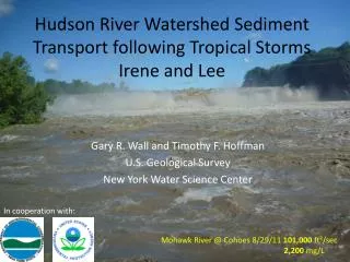
4. Sediment Control Xiao Land Di Reservoir, Yellow River, China Yellow River Reservoir Sediment Release at 9:00am, Clear Water Release at 10:00am, 6/19/2010

5. Scheduled Water Delivery and Pollutant Disposal • Optimal Water Delivery To give an optimal water delivery through irrigation canals to irrigation areas • Optimal Pollutant Discharge To find a optimal discharge to meet regulation for water quality protection, e.g., a tolerable amount of pollutant into water body • Flow-Optimized Discharges • (Scheduled Disposal) Discharging pollutants to waters only during high river flows may mimic the pattern of natural diffuse pollutant loads in waters (such as nutrients or suspended solids exports from the catchment).– Scheduled disposal

6. Applicability of Flow Control Problems • Prevent levee of river from overflowing or breaching during flood season by using the most secure or efficient approach, e.g., operating dam discharge, diverting flood, etc.  Optimal Flood Control  Adaptive Control • Perform an optimally-scheduled water delivery for irrigation to meet the demand of water resource in irrigation canal  Optimal Water Resource Management • To give the best pollutant disposal by controlling pollutant discharge to obey the policy of water quality protection  Best Environmental Management Goal: Real Time Adaptive Control of Open Channel Flow

7. Difficulties in Control of Open Channel Flow • Temporally/spatially non-uniform open channel flow Requires that a forecasting model can predict accurately complex water flows in space and time in single channel and channel network • Nonlinearity of flow control Nonlinear process control, Nonlinear optimization Difficulties to establish the relationship between control actions and responses of the hydrodynamic variables • Requirement of fast flow solver and optimization In case of fast propagation of flood wave, a very short time is available for predicting the flood flow at downstream. Due to the limited time for making decision of flood mitigation, it is crucial for decision makers to have a very efficient forecasting model and a control model.

8. Objectives • Theoretically, • Through adjoint sensitivity analysis, make nonlinear optimization capable of flow control in complex channel shape and channel network in watershed •  Real-Time Nonlinear Adaptive Control Applicable to unsteady river flows • Establish a general simulation-based optimization model for controlling hazardous floods so as to make it applicable to a variety of control scenarios •  Flexible Control System; and a general tool for real-time flow control • Sediment Control: Minimize morphological changes due to flood control actions •  Optimal Control with multiple constraints and objectives • For Engineering Applications, • Integrate the control model with the CCHE1D flow model, • Apply to practical problems

9. Integrated Watershed & Channel Network Modeling with CCHE1D Rainfall-Runoff Simulation Upland Soil Erosion (AGNPS or SWAT) Channel Network and Sub-basin Definition (TOPAZ) Digital Elevation Model (DEM) Channel Network Flow and Sediment Routing (CCHE1D) Principal Features Dynamic Wave Model for Flood Wave Prediction • Hydrodynamic Modeling in Channel Network • Non-uniform Total-Load Transport • Non-equilibrium Transport Model • Coupled Sediment Transport Equations Solution • Bank Erosion and Mass Failure • Several Methods for Determination of Sediment-Related Parameters where Q = discharge; Z=water stage; A=Cross-sectional Area; q=Lateral outflow; =correction factor; R=hydraulic radius n = Manning’s roughness • Boundary Conditions • Initial Conditions (Base Flows) • Internal Flow Conditions for Channel Network

10. CCHE1D Sediment Transport Model Principal Features Non-equilibrium transport of non-uniform sediments • Non-uniform Total-Load Transport • Non-equilibrium Transport Model • Coupled Sediment Transport Equations Solution (Direct Solution Technique) • Bank Erosion and Mass Failure • Several Methods for Determination of Sediment-Related Parameters A=cross-section area; Ctk=section-averaged sediment concentration of size class k; Qtk=actual sediment transport rate; Qt*k=sediment transport capacity; Ls=adaptation length andQlk= lateral inflow or outflow sediment discharge per unit channel length; Ut=section averaged velocity of sediment

11. Control Actions - Available Control Variables in Open Channel Flow • Control lateral flow at a certain location x0: Real-time flow diversion rate q(x0, t)at a spillway • Control lateral flow at the optimal location x: Real-time levee breaching rate q(x, t)at the optimal location • Control upstream discharge Q(0, t): real-time reservoir release • Control downstream stage Z(L, t): real-time gate operation • Control downstream discharge Q(L, t): real-time pump rate control • Control bed friction (roughness n):

12. Objective Function for Flood Control To evaluate the discrepancy between predicted and maximum allowable stages, a weighted form is defined as where T=control duration; L = channel length; t=time; x=distance along channel; Z=predicted water stage; Zobj(x) =maximum allowable water stage in river bank (levee) (or objective water stage); x0= target location where the water stage is protective;  = Dirac delta function Zobj

13. Sensitivity Analysis- Establishing A Relationship between Control Actions and System Variables • Compute the gradient of objective function with respect to control variable 1. Influence Coefficient Method(Yeh, 1986): Parameter perturbation trial-and-error; lower accuracy 2. Sensitivity Equation Method (Ding, Jia, & Wang, 2004) Directly compute the sensitivity ∂X/∂q by solving the sensitivity equations Drawback: different control variables have different forms in the equations, no general measures for system perturbations; The number of sensitivity equations = the number of control variables. Merit: Forward computation, no worry about the storage of codes 3. Adjoint Sensitivity Method (Ding and Wang, 2003) Solve the governing equations and their associated adjoint equations sequentially. Merit: general measures for sensitivity, limited number of the adjoint equations (=number of the governing equations) regardless of the number of control variables. Drawback: Backward computation, has to save the time histories of physical variables before the computation of the adjoint equations.

14. Variational Analysis- to Obtain Adjoint Equations Extended Objective Function where A and Q are the Lagrangian multipliers Necessary Condition on the conditions that Fig. 1: Solution domain

15. Variation of Extended Objective Function where Top width of channel

16. AdjointEquations for the Full Nonlinear Saint Venant Equations According to the extremum condition, all terms multiplied by A and Q can be set to zero, respectively, so as to obtain the equations of the two Lagrangian multipliers, i.e, adjoint equations (Ding & Wang 2003)

17. Adjoint Equations: Linear, Hyperbolic, and of First-Order The obtained adjoint equations are first-order partial differential equations, which can be rewritten into a compact vector form where P represents the source term related to the objective function This adjoint model has two characteristic lines with the following two real and distinct eigenvalues: In the case of a flow in a prismatic open channel, β=1, therefore Wave celerity is the same as the open channel flow. But propagation direction in time is opposite to the flow.

18. Variations of J with Respect to Control Variables – Formulations of Sensitivities Q(0,t) Q(L,t) Lateral Outflow q(x,t) Upstream Discharge Downstream Section Area or Stage Bed Roughness Remarks: Control actions for open channel flows may rely on one control variable or a rational combination of these variables. Therefore, a variety of control scenarios principally can be integrated into a general control model of open channel flow.

19. Optimal Control of Sediment Transport and Morphological Changes • The developed model is coupling an adjoint sensitivity model with a sediment transport simulation model (CCHE1D) to mitigate morphological changes. • Different optimization algorithms have been used to estimate the value of the diverted or imposed sediment along river reach (control actions) to minimize the morphological changes under different practices and applications. Sediment Control Model • Optimization Model • Adjoint sensitivity model • Sediment Transport Simulation Model • CCHE1D

20. A Sediment Transport Model, CCHE1D Overview • Governing equation for the nonequilibrium transport of nonuniform sediment is (1) • In which the depth-average concentration and the sediment transport rate can be expressed as • and Eq. (1) becomes, (2) (3) • The bed deformation is determined with (4) (5) If

21. Objective Function for Sediment Control and Minimization of Morphological Changes (Strong Control Condition) • To evaluate the bed area change, a weighted form is defined as • (6) where f is a measuring function and can be defined as, • (7) • The optimization is to find the control variable q satisfying a dynamic system such that • where Abis satisfied with the sediment continuity equation • Local minimum theory : • Necessary Condition: If q is the true value, then JS(q)=0; • Sufficient Condition: If the Hessian matrix  2JS(q) is positive definite, then qlis a local minimizer of fS. • (8)

22. Optimization Model Consider the equation of morphological change: The objective function for control of morphological changes can be written as and measuring function as, • (9) • (10) where can be taken equal to i.e. the sediment transport capacity. It means that for minimizing morphological change in a cross section, it is needed to make sediment transport rate in the section close to the sediment transport capacity.

23. Variational Analysis for Optimal Control of Morphological Changes An augmented objective function, • (11) where 3is the Lagrangianmultiplier for the sediment transport equation Necessary Condition • (12) on the condition that • (13)

24. Adjoint Equation for Sediment Control Taking the first variation of the augmented objective function, i.e. • (14) (15) • (16) Figure 1. Solution domain By using Green’s theorem and the variation operator δ in time-space domain shown in Fig. (1), the first variation of the augmented function can be obtained • (17) • For minimizing J* , δJ* must be equal zero which means all terms multiplied by δQtmust be set to zero which leads to the following equation, • (18) which is the adjoint equation for the Lagrangianmultiplier λS

25. Boundary Conditions and Transversality Condition Boundary Conditions of Adjoint Equation The contour integral in Eq. (17) needs to be zero so as to satisfy the minimum condition of the performance function J*, namely, Figure 1. Solution domain • (19) • which result in the following boundary conditions for the adjoint equation, • (20)

26. Application of Developed Model To Channel Network – Internal Condition at a Confluence Internal Boundary Condition 2 1 3

27. Sediment Transport Control Actions and Sensitivity Qt(0,t) • Lateral Sediment Discharge Qt(L,t) Lateral Outflow ql • Upstream Sediment Discharge • Downstream Sediment Discharge • In this study,fSis not a function in ql, thus the sensitivity is based on the values of λS.

28. Minimization Procedures • Limited-Memory Quasi-Newton Method (LMQN) Newton-like method, applicable for large-scale computation (with a large number of control parameters), considering the second order derivative of objective function (the approximate Hessian matrix) Algorithms: BFGS (named after its inventors, Broyden, Fletcher, Goldfarb, and Shanno) L-BFGS (unconstrained optimization) L-BFGS-B (bound constrained optimization)

29. Operational Flow Chart Finding optimal control variable using LMQN procedure • Four Major Modules • Flow Solver • Sediment Transport • Sensitivity Solver • Minimization Process

30. Application Optimal Flood Control in Alluvial Rivers and Watersheds

31. Optimal Control of Flood Diversion Rate A Hypothetic Single Channel q(x)= 100m3/s 48 hours 16 hours Storm Event: A Triangular Hydrograph Cross Section

32. Optimal Lateral Outflow and Objective Function (Case 1) Optimal Outflow q Objective function and Norm of gradient of the function Iterations of optimal lateral outflow

33. Comparison of Water Stages in Space and Time (Case 1) Allowable Stage Z0=3.5 Water Stage without Control Optimal Control of Lateral Outflow

34. Thalweg Changes

35. Water Stage and Lateral Discharge The lateral discharge comparison for with and without sediment transport consideration at bed slope The water stage comparison for with and without sediment transport consideration at bed slope

36. Effects of bed slope Slope = Slope = 0.0 Slope = Slope = Comparison of water stages between controlled and uncontrolled states for different bed slopes

37. Lateral Discharges for Different Bed Slopes Slope = Slope = 0.0 Slope = Slope =

38. Optimal Withdrawal Hydrographs under Different Slopes bed material of diameter: 0.127 mm

39. Bed Changes: Slope Effect Fig. 13: The channel bed after the controlled flood has passed for different bed slopes and constant bed material of diameter 0.127 mm

40. Bed Changes: Sediment Size Effect Fig. 14: The channel bed after the controlled flood has passed for different bed materials and constant bed slope

41. Z0=3.5m q1 q2 q3 Optimal Control of Lateral Outflows – Multiple Lateral Outflows (Case 3) Condition of control: Suppose that there are three flood gates (or spillways) in upstream, middle reach, and downstream.

42. Optimal Discharges for Multiple Floodgates

43. Comparison of Thalweg Change

44. Optimal Control of Multiple Lateral Outflows in a Channel Network 1 3 q1(t)=? m 0 0 0 , 4 = 1 L q2(t)=? Z0=3.5m L = 3 1 3 , 0 0 0 m 2 . o N l e n n a h C q3(t)=? m 0 0 5 , 4 = L 2 Compound Channel Section

45. Optimal Lateral Outflow Rates and Objective Function One Diversion Three Diversions Optimal lateral outflow rates at three diversions Comparison of objective function

46. Comparisons of Stages 1 3 m 0 0 0 , 4 = 1 L L = 3 1 3 , 0 0 0 m 2 . o N l e n n a h C m 0 0 5 , 4 = L 2

47. Comparison of Thalweg along Main Channel 3 . 3 3 . 1 I n i t i a l T h a l w e g 4 . 5 C a s e 1 N o C o n t r o l C a s e 1 ( G a t e 1 a t 1 . 5 k m d s ) C a s e 2 ( G a t e 1 a t 2 . 5 k m d s ) C a s e 3 ( G a t e 1 a t 3 . 5 k m d s ) 2 . 9 4 . 0 C a s e 4 ( G a t e 1 a t 4 . 5 k m d s ) C a s e 2 ] m 1 . 5 k m [ 3 . 5 2 . 7 C a s e 1 g e C a s e 2 w C a s e 3 l 3 . 0 a 2 . 5 k m C a s e 3 h ] 2 . 5 T m C a s e 4 [ n o 2 . 5 g i 1 . 5 k m t c a s e 4 e c 3 . 5 k m n w 2 . 3 G a t e 2 u 2 . 5 k m l J a 2 . 0 h 3 . 5 k m n T o i t 4 . 5 k m 4 . 5 k m 2 . 1 c n u 1 . 5 J G a t e 3 1 . 9 1 . 0 I n i t i a l T h a l w e g 0 0 . 5 1 1 . 5 2 2 . 5 3 3 . 5 4 4 . 5 5 5 . 5 N o C o n t r o l C a s e 1 ( G a t e 1 a t 1 . 5 k m d s ) D i s t a n c e [ k m ] C a s e 2 ( G a t e 1 a t 2 . 5 k m d s ) 0 . 5 C a s e 3 ( G a t e 1 a t 3 . 5 k m d s ) C a s e 4 ( G a t e 1 a t 4 . 5 k m d s ) 0 . 0 0 1 2 3 4 5 6 7 8 9 1 0 1 1 1 2 1 3 D i s t a n c e [ k m ]

48. Application Optimal Control of Morphological Changes in Alluvial Rivers and Watersheds

49. Hypothetical Case (1): Dam Removal 20 m Q = 50 m3/s Qs= 10 kg/s Excess Deposition Problem Downstream 1:2 1:2 S = 0.3 % 10 m 3 km S0=0.5 % L=7 km qs = ? Control Objective: To minimize morphological change downstream The inflow and sediment discharge were assumed 50 m3/s and 10 kg/s respectively. Sediment Properties: Uniform sediment of d = 20 mm Simulation time = 1 week Bed load adaptation length = 125 m, suspended load adaptation coefficient = 0.1, and mixing-layer thickness = 0.05 m.

50. Hypothetical Case (1): Model Results