Download
1 / 63
740 likes | 1.08k Views
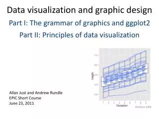
Data visualization and graphic design Part I: The grammar of graphics and ggplot2 Part II: Principles of data visualization. Allan Just and Andrew Rundle EPIC Short Course June 23, 2011. Wickham 2008. Part I: The grammar of graphics and ggplot2. Objectives

E N D
Data visualization and graphic design Part I: The grammar of graphics and ggplot2 Part II: Principles of data visualization Allan Just and Andrew Rundle EPIC Short Course June 23, 2011 Wickham 2008
Part I: The grammar of graphics and ggplot2 Objectives • Revisit the grammar of graphics to describe graphs • Discuss in greater depth the components of the grammar with examples • Customizing plot limits, labels, axes • Exporting for PowerPoint or elsewhere…
R graphics – 3 main "dialects" base: with(airquality, plot(Temp, Ozone)) lattice: xyplot(Ozone ~ Temp, airquality) ggplot2: ggplot(airquality, aes(Temp, Ozone)) + geom_point( )
ggplot2 philosophy Written by Hadley Wickham (Rice Univ.) Extends The Grammar of Graphics (Wilkinson, 2005) All graphs can be constructed by combining specifications with data (Wilkinson, 2005). A specification is a structured way to describe how to build the graph from geometric objects (points, lines, etc.) projected on to scales (x, y, color, size, etc.)
ggplot2 philosophy When you can describe the content of the graph with the grammar, you don’t need to know the name of a particular type of plot… Dot plot, forest plot, Manhattan plot are just special cases of this formal grammar. …a plotting system with good defaults for a large set of components that can be combined in flexible and creative ways…
Building a plot in ggplot2 data to visualize (a data frame) map variables to aesthetic attributes geometric objects – what you see (points, bars, etc) scales map values from data to aesthetic space faceting subsets the data to show multiple plots statistical transformations – summarize data coordinate systems put data on plane of graphic Wickham 2009
A basic ggplot2 graph ggplot(airquality) + geom_point(aes(x = Temp, y = Ozone)) Aesthetics map variables to scales Data Geometric objects to display
Building a plot in ggplot2 ggplot(airquality) + geom_point(aes(x = Temp, y = Ozone)) Aesthetics map variables to scales data to visualize (a data frame) map variables to aesthetic attributes geometric objects – what you see (points, bars, etc) scales map values from data to aesthetic space Data Geometric objects to display Wickham 2009
Building a plot in ggplot2 data to visualize (a data frame) map variables to aesthetic attributes geometric objects – what you see (points, bars, etc) statistical transformations – summarize data scales map values from data to aesthetic space faceting subsets the data to show multiple plots coordinate systems put data on plane of graphic Wickham 2009
Moving beyond templates data(airquality) str(airquality) Let’s do the scatterplot template again…
ggplot2: the parts of speechdata ggplot2 expects a data.frame: Rows: observations Columns: variables diamonds <- data.frame(carat, cut, price) carat cut price 1 0.23 Ideal 326 2 0.21 Premium 326 3 0.23 Good 327 4 0.29 Premium 334 Different layers can work with different data (e.g. a precomputed summary in another data frame)
data in Deducer Drop-down of data.frames currently loaded
ggplot2: the parts of speechaesthetics aesthetics map variables in the data to visual properties of geoms aesthetics include: x, y position color, fill, shape, size,linetype, alpha, group, (depending on the geom)
Different aesthetics for different geoms geom_point() X Y Shape Colour Size Fill Alpha Group
Different aesthetics for different geoms geom_histogram() Y X Colour Fill Size Line Weight Alpha Group Points & lines Areas (inside Polygons)
ggplot2: the parts of speechaesthetics aesthetics map variables in the data to visual properties of geoms Mapping: variable ↔ visual property Done within call to aes(x, y, ...) ggplot(data = airquality) + geom_point(aes(x = Temp, y = Ozone, color = Month)) Color is mapped to month Setting: fixed value → visual property Done outside call to aes(x, y, ...) ggplot(data = airquality) + geom_point(aes(x = Temp, y = Ozone), color = "red") Color is set to "red" – not looking for a variable named "red"
Deducer: mapping vs setting Column of buttons switch between states These two are being mapped Remainder are set (using default settings)
ggplot2: the parts of speechgeometric objects geoms can be simple (point, line, polygon, bar) or built from these components (boxplot, histogram, …)
ggplot2: the parts of speechstatistical transformations Stats are transformations that summarize the data Each stat has a default geom and vice-versa
If you specify a geom you can change the stat
If you specify the stat You can change the geom
ggplot2: the parts of speechscales scales control the mapping between data and aesthetics
But by default – continuous variables map to a color gradient
But now we have an ugly variable name and labels are still bad
We can add in a call to the color scale for discrete vars – "colour hue"
Menus allow us to fix the title and specify meaningful labels
Picking colors – RColorBrewer package colorbrewer.org
ggplot2: the parts of speechfacets facets are subsets of the data to be displayed next to each other as "small multiples" • facet_grid(rowvar ~ columnvar) Use a period to represent no split: facet_grid( . ~ .) • facet_wrap( ~ facetvar) wrap a 1D ribbon of plot panels into a 2D space can specify ncol = #, nrow = # scales control whether shared or independent scales “fixed” (default) Also possible: “free_x”, “free_y”, “free”
Example of facetting for a common x-axis: + facet_grid(datatype ~ ., scales = "free_y") +
Let’s facet our airqualityscatterplot by Month facet_grid() A bug in Deducer – menu for rows and columns are switched in facet_grid in the GUI obvious when we look at our call Also – some issues in implementation of facet_wrap (specification of ncol or nrow) Let’s modify this in code to see how it should work
ggplot2: the parts of speechcoordinate systems "coordinate systems adjust the mapping from coordinates to the 2d plane of the computer screen" Default is coord_cartesian() Could use coord_polar() for cyclical data like a windrose had.co.nz/ggplot2/
Example with coord_flip How do we make horizontal boxplots? Using Ozone from airquality, start with geom_boxplot: Let’s use our old trick to categorize the Month variable happens automatically because boxplots are continuous by discrete. Design will be Ozone ~ as.factor(Month)
ggplot2: the parts of speechcoordinate systems "coordinate systems adjust the mapping from coordinates to the 2d plane of the computer screen" Default is coord_cartesian() This is the best place to zoom in to your data A cautionary example… had.co.nz/ggplot2/
Whereas scale_y_continuous is actually subsetting our data range …
"Other" – a little bit of polish Themes are sets of specifications for adjustable elements like labels, legends, titles, tickmarks, margins, and backgrounds theme_grey() the default look of ggplot2 theme_bw() an alternative in black & white
Note the grey background with light gridlines – default theme_grey()
We can boost base_size to scale all of the figure text up in size
Saving your code/process R is fundamentally a command line language Can't easily reload R code into Deducer's plot builder Deducer specific .ggpfile type to reload the plot builder Plot Builder → File → Save But, saving the R code allows you and others to reuse the code from within R
Saving your output after you hit 'Run' and exit the Plot Builder… The plot window JavaGDhas a File menu with options for saving as: PDF PNG JPG and others … I prefer PNG for PowerPoint, PDF to send to colleagues