Chapter 2: Probability Concepts and Distributions
810 likes | 1.19k Views
Chapter 2: Probability Concepts and Distributions. 2.1 Introduction 2.2 Classical probability 2.3 Probability distribution functions 2.4 Important probability distributions 2.5 Bayesian probability 2.6 Probability concepts and statistics. 2.1.1 Outcomes and Simple Events.

Chapter 2: Probability Concepts and Distributions
E N D
Presentation Transcript
Chapter 2: Probability Concepts and Distributions 2.1 Introduction 2.2 Classical probability 2.3 Probability distribution functions 2.4 Important probability distributions 2.5 Bayesian probability 2.6 Probability concepts and statistics Chap 2-Data Analysis-Reddy
2.1.1 Outcomes and Simple Events A random variable is a numerical description of the outcome of an experiment whose value depends on chance Continuous random variable: one which can take on any value in an interval Discrete random variable: One which can take on only a finite number of values Chap 2-Data Analysis-Reddy
Notions Relevant to Discrete Variables • Trial or random experiment - rolling of a dice • Outcome is the result of a single trial of a random experiment. It cannot be decomposed into anything simpler. For example, getting a {2} when a dice is rolled. • Sample space (or “universe”) is the set of all possible outcomes of a single trial. Rolling of a dice • Eventis the combined outcomes (or a collection) of one or more random experiments. For example, getting a pre-selected number (say, 4) from adding the outcomes of rolling two dices would constitute a simple event: • Complement of a event: set of outcomes in the sample not contained in A. is the complement of above event Chap 2-Data Analysis-Reddy
Classical Concept of Probability Relative frequency is the ratio denoting the fraction of events when success has occurred (after the event) This proportion is interpreted as the long run relative frequency, and is referred to as probability. This is the classical, or frequentist or traditionalist definition apriori or “wise before the event” Bayesian Viewpoint of Probability An approach which allows one to update assessments of probability that integrate prior knowledge (or subjective insights) with observed events Both the classical and the Bayesian approaches converge to the same results as increasingly more data (or information) is gathered. It is when the data sets are small that Bayesian becomes advantageous. Thus, the Bayesian view is not an approach which is at odds with the frequentist approach, but rather adds (or allows the addition of) refinement to it Chap 2-Data Analysis-Reddy
2.2 Classical Probability Permutation P(n,k) is the number of ways that k objects can be selected from n objects with the order being important. Combinations C(n,k) is the number of ways that k objects can be selected from n objects with the order not being important Example 2.2.1. Number of ways in which 3 people from a group of 7 can be seated in a row Chap 2-Data Analysis-Reddy
Factorial problem: special case of combinatorial problemsTable 2.1 Number of combinations for equipment scheduling in a large facility 1-1 0- off 1-on Chap 2-Data Analysis-Reddy
Compound Events Fig. 2.1 Venn diagrams (operations involving two or more events) Sample space Probability of an event Union of two events Intersection of two events Compound event Mutually exclusive events Sub-set Chap 2-Data Analysis-Reddy
2.2.3 Axioms of Probability Let the sample space S consist of two events A and B with probabilities p(A) and p(B) respectively. Then: • probability of any event, say A, cannot be negative: 2.5 • probabilities of all events must be unity (i.e., normalized): 2.6 • probabilities of mutually exclusive events add up: 2.7 if A and B are mutually exclusive Chap 2-Data Analysis-Reddy
2.2.3 Axioms of Probability Some other inferred relations are: • probability of the complement of event A: 2.8 • probability for either A or B (when they are not mutually exclusive) to occur is equal to: 2.9 Chap 2-Data Analysis-Reddy
2.2.4 Joint, marginal and conditional probabilities (a) Joint probabilityof two independent events represents the case when both events occur together: 2.10 if A and B are independent These are called product models. Consider a dice tossing experiment. • event A is the occurrence of an even number, p(A)=1/2. • event B is that the number <= 4, then p(B)=2/3. • Probability that both events occur when a dice is rolled: p(A and B)=1/2 x 2/3 = 1/3. This is consistent with our intuition since events {2,4} would satisfy both the events. Chap 2-Data Analysis-Reddy
. . (b) Marginal probabilityof an event A refers to the probability of A in a joint probability setting. Consider a space containing two events, A and B. Since S can be taken to be the sum of event space and its complement , the probability of A can be expressed in terms of the sum of the disjoint parts of B: 2.11 Notion can be extended to the case of > two joint events. Example 2.2.2. Consider an experiment involving drawing two cards from a deck with replacement. Let event A ={first card is a red one} and event B ={card is between 2 and 8 inclusive} (consistent with intuition) Chap 2-Data Analysis-Reddy
Example 2.3.4. The percentage data of annual income versus age has been gathered from a large population living in a certain region- see Table E2.3.4. Let X be the income and Y the age. The marginal probability of X for each class is simply the sum of the probabilities under each column and that of Y the sum of those for each row. Also, verify that the sum of the marginal probabilities of X and Y sum to 1.00 (so as to satisfy the normalization condition). Chap 2-Data Analysis-Reddy
(c) Conditional probability: There are several situations involving compound outcomes that are sequential or successive in nature. The chance result of the first stage determines the conditions under which the next stage occurs. Such events, called two-stage (or multi-stage) events, involve step-by-step outcomes which can be represented as a probability tree. This allows better visualization of how the probabilities progress from one stage to the next. If A and B are events, then the probability that the event B occurs given that A has already occurred is given by: 2.12 A special but important case is when p(B/A) = p(B). In this case, B is said to be independent of A because the fact that event A has occurred does not affect the probability of B occurring. Chap 2-Data Analysis-Reddy
Example 2.2.4. Two defective bulbs have been mixed with 10 good ones. Let event A= {first bulb is good}, and event B= {second bulb is good}. (a) If two bulbs are chosen at random with replacement, what is the probability that both are good? and . Then: (b) What is the probability that two bulbs drawn in sequence (i.e., not replaced) are good where the status of the bulb can be checked after the first draw? From Eq. 2.12, p(both bulbs drawn are good): Joint Conditional Chap 2-Data Analysis-Reddy
Example 2.2.6. Generating a probability tree for a residential air-conditioning (AC) system. The probability of the indoor conditions being satisfactory: p(S)=0.02+0.27+0.6=0.89 while being not satisfactory: (NS)= 0.08+0.03+0=0.11. Verify that p(S)+p(NS)=1.0. Fig. 2.2 The forward probability tree for the residential air-conditioner when two outcomes are possible (S-satisfactory or NS-not satisfactory) for each of three day-types (VH- very hot, H-hot and NH- not hot). Chap 2-Data Analysis-Reddy
Example 2.2.7. Two-stage experiment There are two boxes with marbles as specified: Box 1: 1 red and 1 white and Box 2: 3 red and 1 green A box is chosen at random and a marble drawn from it. What is the probability of getting a red marble? One is tempted to say that since there are 3 red marbles in total out of 6 marbles, the probability is 2/3. However, this is incorrect, and the proper analysis approach requires that one frame this problem as a two-stage experiment: - first stage is the selection of the box, - second the drawing of the marble. Chap 2-Data Analysis-Reddy
Example 2.2.7. Two-stage experiment (contd.) Table 2.3 Probabilities of various outcomes Fig. 2.3 The first stage of the forward probability tree diagram involves selecting a box (either A or B) while the second stage involves drawing a marble which can be red (R), white (W) or green (G) in color. The total probability of drawing a red marble is 5/8. Chap 2-Data Analysis-Reddy
Fig. 2.4 Probability functions for a discrete random variable involving the outcome of rolling a dice 2.3 Probability Density Functions (pdf) 2.3.1 Density functions • pdf: the probability of a random variable taking different values • The cumulative distribution function (cdf) is the integral of the pdf. It is • the probability that the random variable assumes a value less than or equal to • different values (a) Probability density function (b) Cumulative distribution function Chap 2-Data Analysis-Reddy
Fig. 2.5 Probability density function and its association with probability for a continuous random variable involving the outcomes of hourly outdoor temperatures at Philadelphia, PA during a year. The probability that the temperature will be between 550 and 600 F is given by the shaded area. The axioms of probability (Eqs. 2.5 and 2.6) for the discrete case are expressed for the case of continuous random variables as: • PDF cannot be negative: • Probability of the sum of all outcomes must be unity 2.13 2.14 (a) Density function (b) Probability interpreted as an area Chap 2-Data Analysis-Reddy
The cumulative distribution function (CDF) or F(a) represents the area under f(x) enclosed in the range Fig. 2.6 The cumulative distribution function (CDF) for the PDF shown in Fig. 2.5. Such a plot allows one to easily determine the probability that the temperature is less than 600 F 2.15 Chap 2-Data Analysis-Reddy
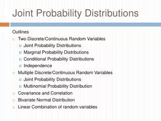
Simultaneous outcomes of multiple random variablesLet X and Y be the two random variables. The probability that they occur together can be represented by a function for any pair of values within the range of variability of the random variables X and Y. This function is referred to as the joint probability density function of X and Y which has to satisfy the following properties for continuous variables: 2.18 2.19 Chap 2-Data Analysis-Reddy
Joint, Marginal and Conditional Distributions • If X and Y are two independentrandom variables, their joint PDF will be the product of their marginal ones: 2.21 Note that this is the continuous variable counterpart of Eq.2.10 which gives the joint probability of two discrete events. • The marginal distributionof X given two jointly distributed random variables X and Y is simply the probability distribution of X ignoring that of Y. This is determined for X as: • Conditional probability distributionof X given that X=x for two jointly distributed random variables X and Y is Chap 2-Data Analysis-Reddy
Example 2.3.1 Determine the value of c so that each of the following functions can serve as probability distribution of the discrete random variable X: (a) One uses the discrete version of Eq. 2.14, i.e., leads to 4c+5c+8c+13c=1 from which c=1/30 (b) Use Eq. 2.14 from which resulting in a=1/3. Chap 2-Data Analysis-Reddy
Example 2.3.2. The operating life in weeks of a high efficiency air filter in an industrial plant is a random variable X having the PDF: • Find the probability that the filter will have an operating life of: • at least 20 weeks • anywhere between 80 and 120 weeks First, determine the expression for the CDF from Eq. 2.14. Since the operating life would decrease with time, one needs to be careful about the limits of integration applicable to this case. Thus, CDF= (a) with x=20, the probability that the life is at least 20 weeks: (b) for this case, the limits of integration are simply modified as follows: Chap 2-Data Analysis-Reddy
2.3.2 Expectations and Moments • Ways by which one can summarize the characteristics of a probability function using a few important measures: • expected value of the first moment or mean: • (analogous to center of gravity) • variance • (analogous to moment of inertia) • Alternative expression • While taking measurements, variance can be linked to errors. The relative erroris often of more importance than the actual error. This has led to the widespread use of a dimensionless quantity called the Coefficient of Variation(CV) defined as the percentage ratio of the standard deviation to the mean: Chap 2-Data Analysis-Reddy
2.3.3 Function of Random Variables The above definitions can be extended to the case when the random variable X is a function of several random variables; for example: 2.27 where the ai coefficients are constants and Xi are random variables. Some important relations regarding the mean: 2.28 Chap 2-Data Analysis-Reddy
2.3.3 Function of Random Variables contd. Similarly there are a few important relations that apply to the variance: 2.29 Again, if the two random variables are independent, 2.30 The notion of covarianceof two random variables is an important one since it is a measure of the tendency of two random variables to vary together. The covariance is defined as: 2.31 where are the mean values of the random variables X1 and X2 respectively. Thus, for the case of two random variables which are not independent, Eq. 2.30 needs to be modified into: 2.32 Chap 2-Data Analysis-Reddy
Example 2.3.5. Let X be a random variable representing the number of students who fail a class. The discrete event form of Eqs. 2.24 and 2.25 is used to compute the mean and the variance: Further: Hence: Chap 2-Data Analysis-Reddy
(a) Skewed to the right (b) Symmetric (c) Skewed to the left Fig. 2.7 Skewed and symmetric distributions (a) Unimodal (b) Bi-modal Fig. 2.8 Unimodal and bi-modal distributions Chap 2-Data Analysis-Reddy
2.4 Important Probability Distributions • Several random physical phenomena seem to exhibit different probability distributions depending on their origin • The ability to characterize data in this manner provides distinct advantages to the analysts in terms of: - understanding the basic dynamics of the phenomenon, - in prediction and in confidence interval specification, - in classification and in hypothesis testing Such insights eventually allow better decision making or sounder structural model identification since they provide a means of quantifying the random uncertainties inherent in the data. Chap 2-Data Analysis-Reddy
Fig. 2.9 Genealogy between different important probability distribution functions. Those that are discrete functions are represented by “D” while the rest are continuous functions. (Adapted with modification from R.E. Lave, Jr. of Stanford University) Chap 2-Data Analysis-Reddy
2.4.2 Distributions for Discrete Variables • Bernouilli process. Experiment involving repeated trials where : - only two complementary outcomes are possible: “success” or “failure” - if the successive trials are independent, and - if the probability of success p remains constant from one trial to the next. (b)Binomial distribution applies to the binomial random variable taken to be the number of successes in n Bernouilli trials. It gives the probability of x successes in n independent trials: 2.4.1a with mean: = (n.p) and variance 2.4.1b For large values of n, it is more convenient to refer to Table A1 which applies not to the PDF but to the corresponding cumulative distribution functions, referred to here as Binomial probability sumsdefined as: Chap 2-Data Analysis-Reddy
Example 2.4.1. Let x be the number of heads in n=4 independent tosses of a coin. - mean of the distribution = (4).(1/2) = 2, - variance = (4).(1/2).(1-1/2) = 1. - From Eq. 2.33a, the probability of two successes (x=2) in four tosses = Chap 2-Data Analysis-Reddy
Example 2.4.2. The probability that a patient recovers from a type of cancer is 0.6. If 15 people are known to have contracted this disease, then one can determine probabilities of various types of cases using Table A1. Let X be the number of people who survive. • The probability that at least 5 survive is: (b) The probability that there will be 5 to 8 survivors is: (c) The probability that exactly 5 survive: Chap 2-Data Analysis-Reddy
Fig. 2.10 Plots for the Binomial distribution illustrating the effect of probability of success p with X being the probability of the number of “successes” in a total number of n trials. Chap 2-Data Analysis-Reddy
(c) Geometric Distribution Applies to physical instances where one would like to ascertain the time interval for a certain probability event to occur the first time (which could very well destroy the physical system). • Consider “n” to be the random variable representing the number of trials until the event does occur and note that if an event occurs the first time during the nth trial then it did not occur during the previous (n-1) trials. Then, the geometric distribution is given by: n=1,2,3,… 2.34a • Recurrence time: time between two successive occurrences of the same event. Since the events are assumed independent, the mean recurrence time (T) between two consecutive events is simply the expected value of the Bernouilli distribution: 2.34b Chap 2-Data Analysis-Reddy
Example 2.4.3Using geometric PDF for 50 year design wind problems The design code for buildings in a certain coastal region specifies the 50-yr wind as the “design wind”, i.e., a wind velocity with a return period of 50 years or, one which may be expected to occur once every 50 years. What are the probabilities that: (i) the design wind is encountered in any given year. • From eq. 2.34b Fig. 2.11 Geometric distribution G(x;0.02) where the random variable is the number of trials until the event occurs, namely the “50 year design wind” at the coastal location • (ii) the design wind is encountered during the fifth year • of a newly constructed building (from Eq. 2.34a): • (iii) the design wind is encountered within the first 5 years: Chap 2-Data Analysis-Reddy
Poisson experiments are those that involve the number of outcomes of a random variable X which occur per unit time (or space); in other words, as describing the occurrence of isolated events in a continuum. A Poisson experiment is characterized by: (i) independent outcomes (also referred to as memoryless), (ii) probability that a single outcome will occur during a very short time is proportional to the length of the time interval, and (iii) probability of more than one outcome occurs during a very short time is negligible. These conditions lead to the Poisson distribution which is the limit of the Binomial distribution in such a way that the product (n.p) = remains constant. x=0,1,2,3… 2.37awhere is called the “mean occurrence rate”, i.e., the average number of occurrences of the event per unit time (or space) interval t. A special feature of this distribution is that its mean or average number of outcomes per time t and its variance are such that 2.37b (d) Poisson Distribution Chap 2-Data Analysis-Reddy
Applications of the Poisson distribution are widespread: - the number of faults in a length of cable, - number of cars in a fixed length of roadway - number of cars passing a point in a fixed time interval (traffic flow), - counts of -particles in radio-active decay, - number of arrivals in an interval of time (queuing theory), - the number of noticeable surface defects found on a new automobile,...Example 2.4.6. During a laboratory experiment, the average number of radioactive particles passing through a counter in 1 millisecond is 4. What is the probability that 6 particles enter the counter in any given millisecond?Using the Poisson distribution function (Eq. 2.37a) with x=6 and :Example 2.4.7. The average number of planes landing at an airport each hour is 10 while the maximum number it can handle is 15. What is the probability that on a given hour some planes will have to be put on a holding pattern? From Table A2, with : Chap 2-Data Analysis-Reddy
Table A2: Cumulative probability values for the Poisson distribution Chap 2-Data Analysis-Reddy
Fig. 2.12 Poisson distribution for the number of storms per year where . • Example 2.4.8. Using Poisson PDF for assessing storm frequency • Historical records at Phoenix, AZ indicate that on an average there are 4 dust storms per year. Assuming a Poisson distribution, compute the probabilities of the following events (use Eq. 2.37a): • that there would not be any storms • at all during a year: • (b) the probability that there will be four • storms during a year: • Note that the though the average is four, the probability of actually encountering four storms in a year is less than 20%. Chap 2-Data Analysis-Reddy
2.4.2 Distributions for Discrete Variables • Gaussian distributionor normal error function is the best known of all continuous distributions. It is a special case of the Binomial distribution with the same values of mean and variance but applicable when is sufficiently large (n>30). It is a two-parameter distribution given by: 2.38a where are the mean and standard deviation respectively • Its name stems from an erroneous earlier perception that it was the natural pattern and that any deviation required investigation. • Nevertheless, it has numerous applications in practice and is the most important of all distributions studied in statistics. • It is used to model events which occur by chance such as variation of dimensions of mass-produced items during manufacturing, experimental errors, variability in measurable biological traits such as people’s height • Applies in situations where the random variable is the result of a sum of several other variable quantities acting independently on the system Chap 2-Data Analysis-Reddy
Fig. 2.13 Normal or Gaussian distributions with the same mean of 10 but different standard deviations. The distribution flattens out as the standard deviation increases. In problems where the normal distribution is used, it is more convenient to • standardize the random variable into a new random variable with mean zero • and variance of unity • This results in the standard normal curve or z-curve: Chap 2-Data Analysis-Reddy
In actual problems the standard normal distribution is used to determine the probability of the variate having a value within a certain interval, say z between z1 and z2. Then Eq.2.38a can be modified into: 2.38cThe shaded area in Table A3 permits evaluating the above integral, i.e., determining the associated probability assuming Note that for z=0, the probability given by the shaded area is equal to 0.5. Not all texts adopt the same format in which to present these tables, Chap 2-Data Analysis-Reddy
Table A3. The standard normal distribution (cumulative z curve areas) Chap 2-Data Analysis-Reddy
Example 2.4.9.Graphical interpretation of probability using the standard normal table Resistors have a nominal value of 100 ohms but their actual values are normally distributed with a mean = 100.6 ohms and standard deviation = 3 ohms. Find the percentage of resistors that will have values: • higher than the nominal rating. The standard normal variable z(x = 100)= (100-100.6)/3 = -0.2. From Table A3, this corresponds to a probability of (1-0.4207)=0.5793 or 57.93%. (ii) within 3 ohms of the nominal rating (i.e., between 97 and 103 ohms). The lower limit z1 = (97 - 100.6)/3 = -1.2, and the tabulated probability from Table A3 is p(z=-1.2)=0.1151 (as illustrated in Fig.2.14). The upper limit is: z2 = (103 - 100.6)/3 = 0.8. - First determine the probability about the negative value symmetric about 0, i.e., p(z=-0.8)= 0.2119 (shown in Fig.2.14b). - Since the total area under the curve is 1.0, p(z=0.8)= 1.0-0.2119=0.7881. - Finally, the reqd probability p(-1.2< z < 0.8) = (0.7881 - 0.1151) = 0.6730 or 67.3%. Fig. 2.14 Chap 2-Data Analysis-Reddy
(b) Student t Distribution One important application of the normal distribution is that it allows making statistical inferences about population means from random samples. In case the random samples are small (n< 30), then the t-student distribution, rather than the normal distribution, should be used. If one assumes that the sampled population is approximately normally distributed, then the random variable has the Student t-distribution where s is the sample standard deviation and is the degrees of freedom = (n-1). Fig. 2.15 Comparison of the normal (or Gaussian) z curve to two Student –t curves with different degrees of freedom (d.f.). As the d.f increase, the PDF for the Student-t distribution flattens out and deviates increasingly from the normal distribution Chap 2-Data Analysis-Reddy
(c) Lognormal Distribution Skewed distribution appropriate for non-negative outcomes: - which are the product of a number of quantities - captures the non-negative nature of many variables occuring in practice If a variate X is such that log(X) is normally distributed, then the distribution of X is said to be lognormal. With X ranging from , log(X) would range from 0 to It is characterized by two parameters, the mean and variance =0 elsewhere Eq. 2.39 Fig. 2.16 Lognormal distributions for different mean and standard deviation values Chap 2-Data Analysis-Reddy
Lognormal failure laws apply for modeling systems:- when degradation in life is proportional to previous amount (ex.: electri transformers)- flood frequency (civil engg), crack growth or wear (mechanical engg), and pollutants produced by chemical plants and threshold values for drug dosage (env. engg). Example 2.4.11. Using lognormal distributions for pollutant concentrationsConcentration of pollutants produced by chemical plants is known to resemble lognormal distributions and is used to evaluate issues regarding compliance of government regulations. The concentration of a certain pollutant, in parts per million (ppm), is assumed lognormal with parameters What is the probability that the concentration exceeds 10 ppm?One can use Eq. 2.39, or simpler still, use the z tables (Table A3) by suitable transformations of the random variable: Chap 2-Data Analysis-Reddy