Download

1 / 35
350 likes | 505 Views
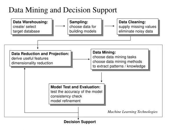
OLAP and Decision Support. Chapter 25, Part A. Introduction. Increasingly, organizations are analyzing current and historical data to identify useful patterns and support business strategies.

E N D
OLAP and Decision Support Chapter 25, Part A
Introduction • Increasingly,organizations are analyzing current and historical data to identify useful patterns and support business strategies. • Emphasis is on complex, interactive, exploratory analysis of very large datasets created by integrating data from across all parts of an enterprise; data is fairly static. • Solving modern business problems such as market analysis requires query-centric database schemas that are multidimensional.
Three Complementary Trends • Data Warehousing: Consolidate data from many sources in one large repository. • Loading, periodic synchronization of replicas. • Semantic integration. • OLAP: • Complex SQL queries and views. • Queries based on spreadsheet-style operations and “multidimensional” view of data. • Interactive and “online” queries. • Data Mining: Exploratory search for interesting trends and anomalies. (Another lecture!)
OLAP versus OLTP OLTP( Online Transaction Proccess ) is used to run the business operations of a company such as inventory management and order processing. On the other hand, OLAP works with data that is geared towards decision making, esp. long-term strategic decisions.
8 10 10 pid 11 12 13 30 20 50 25 8 15 1 2 3 timeid Multidimensional Data Model Fact Table -> timeid locid sales pid • Collection of numeric measures, which depend on a set of dimensions. • E.g., measure Sales, dimensions Product (key: pid), Location (locid), and Time (timeid). Slice locid=1 is shown: locid
Why Multidimensional Data Model • Traditional relational databases, as well as spreadsheets , are based on two dimensional model such as # of customers by region. • However, a telecommunication company analyst may not be interested just determining the number of the phone customers in a single state such as PA.
Why Multidimensional Data Model • For ex, the analyst might like to determine the number of customers who subscribed to both home and wireless service in the past year. • The scenario may become more complicated as more dimensions are added. • The analyst would have to access data in different tables and perform complex table joins, a task would be beyond the capabilities of ordinary user.
Why Multidimensional Data Model Three dimensional model Region Product Time
What is OLAP? • OLAP is an analytical technique that combines data access tools with an analytical database engine. In contrast to the simple rows and columns structure of relational databases, OLAP uses a multi-dimensional view of data. OLAP uses calculations and transformations to perform its analytical tasks. There are two types of OLAP systems architectures ;
MOLAP vs ROLAP • In Multidimensional OLAP ( MOLAP ), data is stored in a special OLAP database server, after being extracted from various sources, in pre-aggregated cubic format. In contrast to this approach, Relational OLAP ( ROLAP ) does not use an intermediate server because it can work directly against the relational database.
MOLAP vs ROLAP • MOLAP performs well with 10 dimensions while ROLAP can scale considerably higher. ROLAP ‘s advantage is that it can work directly relational database and it is not limited by 10 dimensions but it places a heavy load on the server which makes it much slower and ROLAP is expensive to maintain.
Dimension and Fact tables TIMES (Dimension) timeid date week month quarter year holiday_flag (Fact table) pid timeid locid sales SALES PRODUCTS LOCATIONS pid pname category price locid city state country (Dimension table) (Dimension table) • The main relation, which relates dimensions to a measure, is called the fact table. Each dimension can have additional attributes and an associated dimension table. • E.g., Products(pid, pname, category, price) • Fact tables are much larger than dimensional tables.
Dimension Hierarchies • For each dimension, the set of values can be organized in a hierarchy: PRODUCT TIME LOCATION year quarter country category week month state pname date city
OLAP Queries • Influenced by SQL and by spreadsheets. • A common operation is to aggregate a measure over one or more dimensions. • Find total sales. • Find total sales for each city, or for each state. • Find top five products ranked by total sales. • Roll-up: Aggregating at different levels of a dimension hierarchy. • E.g., Given total sales by city, we can roll-up to get sales by state.
OLAP Queries • Drill-down: The inverse of roll-up. • E.g., Given total sales by state, can drill-down to get total sales by city. • E.g., Can also drill-down on different dimension to get total sales by product for each state. • Pivoting: Aggregation on selected dimensions. • E.g., Pivoting on Location and Time yields this cross-tabulation: WI CA Total 63 81 144 1995 • Slicing and Dicing: Equality • and range selections on one • or more dimensions. 38 107 145 1996 75 35 110 1997 176 223 339 Total
OLAP Queries Dice Slice Slicing and dicing basically are used for viewing different range of different dimension selection.
Comparison with SQL Queries • The cross-tabulation obtained by pivoting can also be computed using a collection of SQL queries: SELECT SUM(S.sales) FROM Sales S, Times T, Locations L WHERE S.timeid=T.timeid AND S.timeid=L.timeid GROUP BY T.year, L.state WI CA Total 63 81 144 1995 This query generates the entries in the body of the chart( outlined by the dark lines ) 38 107 145 1996 75 35 110 1997 176 223 339 Total
Comparison with SQL Queries SELECT SUM(S.sales) FROM Sales S, Times T WHERE S.timeid=T.timeid GROUP BY T.year The summary column on the right is generated by this query SELECT SUM(S.sales) FROM Sales S, Location L WHERE S.timeid=L.timeid GROUP BY L.state The summary row at the bottom is generated by this query SELECT SUM(S.sales) FROM Sales S, Location L WHERE S.locid=L.locid The cumulative sum in the bottom corner of the chart.
The CUBE Operator • Generalizing the previous example, if there are k dimensions, we have 2^k possible SQL GROUP BY queries that can be generated through pivoting on a subset of dimensions. • GROUP BY CUBE SELECT T.year, L.state, SUM (S.sales) FROM Sales S, Times T, Locations L WHERE S.timeid = T.timeid AND S.locid=L.locid GROUP BY CUBE( T.year, L.state )
The CUBE Operator The Result of GROUP BY CUBE on Sales
The CUBE Operator CUBE pid, locid, timeid BY SUM Sales • This query rolls up the table Sales on all eight subsets of the set {pid, locid, timeid}. It is equivalent to eight queries of the form: SELECT SUM(S.sales) FROM Sales S GROUP BY grouping list • grouping list is some set of the set {pid, locid, timeid}
Implementation Issues • New indexing techniques: Bitmap indexes, Join indexes, array representations, compression, precomputation of aggregations, etc. • E.g., Bitmap index: sex custid name sex rating rating Bit-vector: 1 bit for each possible value. Many queries can be answered using bit-vector ops! F M
Join Indexes • Consider the join of Sales, Products, Times, and Locations, possibly with additional selection conditions (e.g., country=“USA”). • A join index can be constructed to speed up such joins. The index contains [s,p,t,l] if there are tuples (with sid) s in Sales, p in Products, t in Times and l in Locations that satisfy the join (and selection) conditions. • Problem: Number of join indexes can grow rapidly. • A variation addresses this problem: For each column with an additional selection (e.g., country), build an index with [c,s] in it if a dimension table tuple with value c in the selection column joins with a Sales tuple with sid s; if indexes are bitmaps, called bitmapped join index.
Bitmapped Join Index TIMES timeid date week month quarter year holiday_flag • Consider a query with conditions price=10 and country=“USA”. Suppose tuple (with sid) s in Sales joins with a tuple p with price=10 and a tuple l with country =“USA”. There are two join indexes; one containing [10,s] and the other [USA,s]. • Intersecting these indexes tells us which tuples in Sales are in the join and satisfy the given selection. (Fact table) pid timeid locid sales SALES PRODUCTS LOCATIONS pid pname category price locid city state country
Querying Sequences in SQL:1999 • Trend analysis is difficult to do in SQL-92: • Find the % change in monthly sales • Find the top 5 product by total sales • Find the trailing n-day moving average of sales • The first two queries can be expressed with difficulty, but the third cannot even be expressed in SQL-92 if n is a parameter of the query. • The WINDOW clause in SQL:1999 allows us to write such queries over a table viewed as a sequence (implicitly, based on user-specified sort keys)
The WINDOW Clause SELECT L.state, T.month, AVG(S.sales) OVER W AS movavg FROM Sales S, Times T, Locations L WHERE S.timeid=T.timeid AND S.locid=L.locid WINDOW W AS (PARTITION BY L.state ORDER BY T.month RANGE BETWEEN INTERVAL `1’ MONTH PRECEDING AND INTERVAL `1’ MONTH FOLLOWING) • This example shows moving average of sales over 3 months • Let the result of the FROM and WHERE clauses be “Temp”. • (Conceptually) Temp is partitioned according to the PARTITION BY clause. • Similar to GROUP BY, but the answer has one row for each row in a partition, not one row per partition!
The Window Clause • Each partition is sorted according to the ORDER BY clause. • For each row in a partition, the WINDOW clause creates a “window” of nearby (preceding or succeeding) tuples. • Can be value-based, as in example, using RANGE • Can be based on number of rows to include in the window, using ROWS clause • The aggregate function is evaluated for each row in the partition using the corresponding window.
The Window Clause • In the example, the window for a row includes the row itself plus all rows whose “month” value is within a month value is within a month before or after; therefore, a row whose month value is June 2002 has a window containing all rows with month equal to May, June, and July 2002.
Top N Queries • If you want to find the 10 (or so) cheapest cars, it would be nice if the DB could avoid computing the costs of all cars before sorting to determine the 10 cheapest. • Idea: Guess at a cost c such that the 10 cheapest all cost less than c, and that not too many more cost less. Then add the selection cost<c and evaluate the query. • If the guess is right, great, we avoid computation for cars that cost more than c. • If the guess is wrong, need to reset the selection and recompute the original query.
Top N Queries SELECT P.pid, P.pname, S.sales FROM Sales S, Products P WHERE S.pid=P.pid AND S.locid=1 AND S.timeid=3 ORDER BY S.sales DESC OPTIMIZE FOR 10 ROWS • OPTIMIZE FOR construct is not in SQL:1999! • Cut-off value c is chosen by optimizer. SELECT P.pid, P.pname, S.sales FROM Sales S, Products P WHERE S.pid=P.pid AND S.locid=1 AND S.timeid=3 AND S.sales > c ORDER BY S.sales DESC
Online Aggregation • Consider an aggregate query, e.g., finding the average sales by state. Can we provide the user with some information before the exact average is computed for all states? • Can show the current “running average” for each state as the computation proceeds. • Even better, if we use statistical techniques and sample tuples to aggregate instead of simply scanning the aggregated table, we can provide bounds such as “the average sales for Wisconsin is 2000$±102 with 95% probability. • Should also use nonblocking algorithms!
Online Aggregation An algorithm is said to block if it does not produce output tuples until it has consumed all its input tuples. For example, the sort-merge join algorithm blocks because sorting requires all input tables before determining the first output tuple. Hash join is preferable instead of sort-merge join for online aggregation.
Summary • Decision support is an emerging, rapidly growing subarea of databases. • Involves the creation of large, consolidated data repositories called data warehouses. • Warehouses exploited using sophisticated analysis techniques: complex SQL queries and OLAP “multidimensional” queries (influenced by both SQL and spreadsheets). • New techniques for database design, indexing, view maintenance, and interactive querying need to be supported.