Download
1 / 26
260 likes | 431 Views
Crystallography without Crystals and the Potential of Imaging Single Molecules. John Miao Stanford Synchrotron Radiation Laboratory Stanford Linear Accelerator Center. The Phase Problem. Detector. Coherent Beam. Atoms. The trivial phases:.

E N D
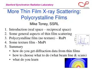
Crystallography without Crystals and the Potential of Imaging Single Molecules John Miao Stanford Synchrotron Radiation Laboratory Stanford Linear Accelerator Center
The Phase Problem Detector Coherent Beam Atoms The trivial phases:
Oversampling: Sampling at Twice of the Bragg-peak Frequency Miao, Sayre & Chapman, J. Opt. Soc. Am. A 15, 1662 (1998). Miao & Sayre, Acta Cryst. A 56, 596 (2000).
The Oversampling Method Eq. (2) > 2: the phase information exists inside the diffraction intensity!
Multiple Solutions 1D Case: ( 2N multiple solutions) 2D & 3D Case: (No multiple solutions) Mathematically, 2D and 3D polynomials usually can not be factorized. Bruck & Sodin, Opt. Commun. 30, 304 (1979).
Coherence Requirements of the Oversampling Method Oversampling vs. spatial coherence: sample size : Oversampling vs. temporal coherence: : desired resolution Miao et al., Phys. Rev. Lett.89, 088303 (2002).
An Iterative Algorithm (I) with > 5 (II) (III) = 0 ) FFT-1( = (IV) (V) ) = FFT( (VI) Adopt from (VII) Fienup, Appl. Opt. 21, 2758 (1982). Miao et al., Phys. Rev. B67, 174104 (2003).
The First Experiment of Crystallography without Crystals (a) A SEM image (b) An oversampled diffraction pattern (in a logarithmic scale) from (a). (c) An image reconstructed from (b). (d) The convergence of the reconstruction. Miao, Charalambous, Kirz, Sayre, Nature 400, 342 (1999).
Phase Retrieval as a Function of the oversampling ratio () = 5 (180 x 180 pixels) = 4 (160 x 160 pixels) = 2.6 (130 x 130 pixels) = 1.9 (110 x 110 pixels) Miao et al., PRB, in press.
Imaging Buried Nanostructures (a) A SEM image of a double-layered sample made of Ni (~2.7 x 2.5 x 1 m3) (b) A coherent diffraction pattern from (a) (the resolution at the edge is 8 nm) (c) An image reconstructed from (b) Miao et al., Phys. Rev. Lett.89, 088303 (2002).
3D Imaging of Nanostructures The reconstructed top pattern The reconstructed bottom pattern An iso-surface rendering of the reconstructed 3D structure
Determining the Absolute Electron Density of Disordered Materials at Sub-10 nm Resolution (a) A coherent diffraction pattern from a porous silica particle (b) The reconstructed absolute electron density (c) The absoluteelectron density distribution within a 100 x 100 nm2 area Miao et al., Phys. Rev. B,in press.
Imaging E. Coli Bacteria (a) Light and fluorescence microscopy images of E. Coli labeled with manganese oxide (b) A Coherent X-ray diffraction pattern from E. Coli Miao et al., Proc. Natl. Acad. Sci. USA 100, 110 (2003). (c) An image reconstructed from (b).
3D Electron Diffraction Microscopy Electron gun Aperture Lens Sample Detector
Computer Simulation of Imaging a 3D Nanocrystal ([Al12Si12O48]8) with coherent electron diffraction Si Al O (b) One of the 29 diffraction patterns (the 0 projection), SNR = 3 (a) A section (0.5 Å thick) viewed along [100] at z = 0 (c) The reconstructed section (0.5 Å thick) of the nanocrystal viewed along [100] at z = 0 Miao et al., Phys. Rev. Lett. 89, 155502 (2002).
Peak and Time Averaged Brightness of the LCLS and Other Facilities Operating or Under Construction TESLA TESLA
A Potential Set-up for ImagingSingle Biomolecules Using X-FELs X-ray Lens Molecular Spraying Gun X-FEL Pulses CCD
Two Major Challenges Radiation Damage Solemn & Baldwin, Science 218, 229 (1982). Neutze et al.,Nature 400, 752 (2000). When an X-ray pulse is short enough ( < 50 fs), a 2D diffraction pattern could berecorded from a molecule before it is destroyed. Orientation Determination Use the methods developed in cryo-EM to determine the molecular orientation based on many 2D diffraction patterns. Crowther, Phil. Trans. Roy. Soc. Lond. B. 261, 221 (1971). Use laser fields to physically align each molecule. Larsen et al., Phys. Rev. Lett. 85, 2470 (2000).
An Oversampled 3D Diffraction Pattern Calculated from 3 x 10⁵ Rubisco Protein Molecules • One section of the oversampled 3D • diffractionpattern with Poisson noise (b) Top view of (a)
The ReconstructedElectron Density from the Oversampled Diffraction Pattern The 3D electron density map of a rubisco molecule The active site of the molecule The reconstructed 3D electron density map The reconstructed active site Miao, Hodgson & Sayre, Proc. Natl. Acad. Sci. USA98, 6641 (2001).
Summary • Proposed a theoretical explanation to the oversampling method. • Carried out the first experiment of crystallography without crystals. • Opened a door to atomic resolution 3D X-ray diffraction microscopy. • Proposed 3D electron diffraction microscopy for achieving sub-atomic resolution. • Future application with the LCLS – imaging non-crystalline materials • nanocrystals, and large biomoleucles.
Acknowledgements • B. Johnson, D. Durkin, K. O. Hodgson, SSRL • J. Kirz, D. Sayre, SUNY at Stony Brook • R. Blankenbecler, SLAC • D. Donoho, Stanford University • C. Larabell, UC San Francisco & LBL • M. LeGros, E. Anderson, M. A. O’Keefe, LBL • B. Lai, APS • T. Ishikawa, Y. Nishino, Y. Kohmura, RIKEN/SPring-8 • J. Amonette, PNL • O. Terasaki, Tohoku University
Schematic Layout of the Experimental Instrument 25.4 mm 12.7 mm 743 mm Sample Pinhole X-rays Corner Beamstop Photodiode CCD
Experimental Demonstration of Electron Diffraction Microscopy Left: The reconstructed DWNT image; Right: A structure model of the DWNT. The recorded diffraction pattern from a DWNT. Zuo et al., Science 300, 1419 (2003).