Classifying Antagonistic Interactions
Classifying Antagonistic Interactions. Classifying Antagonistic Interactions. Wildebeest. Guanaco. Classifying Antagonistic Interactions. Greya piperella. Sea lamprey. Classifying Antagonistic Interactions. Classifying Antagonistic Interactions. Crossbill.
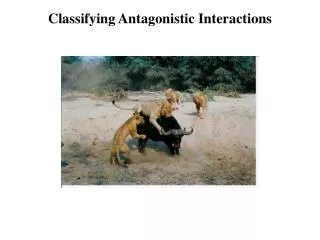

Classifying Antagonistic Interactions
E N D
Presentation Transcript
Classifying Antagonistic Interactions Wildebeest Guanaco
Classifying Antagonistic Interactions Greya piperella Sea lamprey
Classifying Antagonistic Interactions Crossbill
Antagonistic Interactions: functional definitions Predators – Inevitably kill their prey. Attack and kill many different prey individuals Grazers – Generally don’t kill prey (at least in the short term). Attack a large number of prey individuals over their lifetime Parasites – Generally don’t kill prey (at least in the short term). Attack only one, or very few individuals during the course of their lives Parasitoids – Inevitably kill their prey. Attack only one, or very few individuals during the course of their lives
Functional Predators Brook Trout Salvelinus fontinalis Masked ShrewSorex cinereus Mountain lion Puma concolor Dragonfly Diphlebia lestoides
What role does predation play in regulating population densities? Lepus americanus (Snowshoe hare) Lynx canadensis (Lynx)
What role does predation play in regulating population densities?
Population cycles of Lynx and Hare Data from Hudson’s Bay Company pelt records Are these cycles in lynx and hare densities the product of predation?
The Lotka-Volterra Predation Model Alfred James Lotka(1880 - 1949) Vito Volterra(1860-1940)
The Lotka-Volterra Predation Model Prey Predator is the per capita impact of the predator on the prey (-) is the per capita impact of the prey on the predator (+) q is the predator death rate (assumes a specialist predator)
What are the equilibria? Prey Predator Here we see that P = 0 is one equilibrium, but there is also another: Here we see that N = 0 is one equilibrium, but there is also another: Solving for the prey equilibrium actually gives us an answer in terms of the predator! Solving for the predator equilibrium actually gives us an answer in terms of the prey!
Are these equilibria ever reached? (in this example, r = and q = ) Time series plots Phase plots Equilibrium Equilibrium Prey Population density Predator density Predator Equilibrium Prey Predator density Population density Predator Equilibrium Time Prey density The model always produces cycles in population densities!
These cycles are neutrally stable Prey • Properties of neutrally stable cycles • Amplitude remains constant • Amplitude determined solely by initial deviation from equilibrium • Sensitive to disturbance Population density Predator Prey Population density Predator Time
Sensitive to disturbance Prey Population density Predator density Predator Disturbance Prey density Time • Cycle amplitude is determined solely by initial deviation from equilibrium • Disturbances can qualitatively change cyclical dynamics
Summary of the Lotka-Volterra predation model • The only possible behavior is population cycles • Cycles are ‘neutrally stable’ • Cycle amplitude depends solely on initial population sizes • Stable equilibria are not possible • At some times, predators effectively regulate prey density • (at others, they do not)
Practice problem 1967 • In 1967, two bird species were introduced onto an island. • The depth of an individual’s beak determines the size of seeds it can consume • The distribution of beak depths in the two species was measured in 1967 and again in 2008 and is shown at left • Develop a hypothesis to explain this data. Species 1 Species 2 # Birds Beak Depth 2008 Species 1 Species 2 # Birds Beak Depth
Cycles? Yes; Neutrally stable? No Are the model assumptions incorrect?
Model assumptions • Growth of the prey is limited only by predation (i.e., no K) • The predator is a specialist that can persist only in the presence of this single prey item • Individual predators can consume an infinite # of prey • Predator and prey encounter one another at random (N*P terms)
Adding prey density dependence Prey Predator Prey density dependence
What is the effect of incorporating prey K? K=10 Prey Predator density Population density Predator K=10 Predator Population density Predator density Prey Time Prey density A stable equilibrium population size is always reached!
Results of adding prey density dependence • Population cycles are no longer neutrally stable • Populations always evolve to a single stable equilibrium • This equilibrium is characterized by a prey population density well below carrying capacity • Suggests that predators could be effective at regulating prey density Predator density Predator density Prey density
Adding limits to predator consumption The original Lotka-Volterra model assumes a ‘Type I Functional Response’ is the slope of this line # of prey eaten per predator Prey density But real predators cannot eat an infinite # of prey!
The Type II Functional Response Type I # of prey eaten per predator Type II Prey density The Type II Functional Response assumes that predators get full!
The Type III Functional Response Type I Type III # of prey eaten per predator Prey density The Type III Functional Response assumes that predators: A) Develop a search image or B) Switch to a prey item as it becomes common
Dynamics with non-linear functional responses Type I # of prey eaten per predator Type II Type I dynamics Prey density Predator density Prey density
Type II Dynamics Prey Predator Prey eaten per predator Population density Population density Prey eaten per predator Increasing predator saturation Population density Prey eaten per predator Prey density Time
Impacts of saturating functional response • Decreases the predators ability to effectively control the prey population • Leads to periodic ‘outbreaks’ in prey population density • Prey outbreaks lead to predator outbreaks • The result can be repeated population outbreaks and crashes, ultimately leading to the extinction of both species
Combining prey K with the Type II functional response Population dynamics Functional response K=10 Prey Predator Prey eaten per predator Population density K=10 Population density Prey eaten per predator Increasing predator saturation K=10 Population density Prey eaten per predator Prey density Time
Combining prey K with the Type II functional response Population dynamics Functional response K=25 Prey eaten per predator Population density K=20 Population density Prey eaten per predator Decreasing prey carrying capacity K=15 Predator Prey Population density Prey eaten per predator Prey density Time
Summarizing the interaction between prey K and saturating predator functional response • Rapidly saturating predator functional responses destabilize population densities • Prey density dependence stabilizes population densities • Whether predator-prey interactions are stable depends on the relative strengths of: • - Prey density dependence • - Predator saturating response
The “paradox of enrichment” results from the interaction of prey K and a saturating predator functional response Carrying capacity increased Population density Time Increasing the carrying capacity of the prey, say through winter feeding, actually destabilizes the system!
Summary of Predator-Prey Models • Predators can control prey population densities • Often, this occurs through population cycles • Cycles are stabilized by strong prey density dependence • Cycles are destabilized by saturating functional responses
EXAM 2 RESULTS Average: 159 points or 79.5% # Students Points