Download
1 / 47

E N D
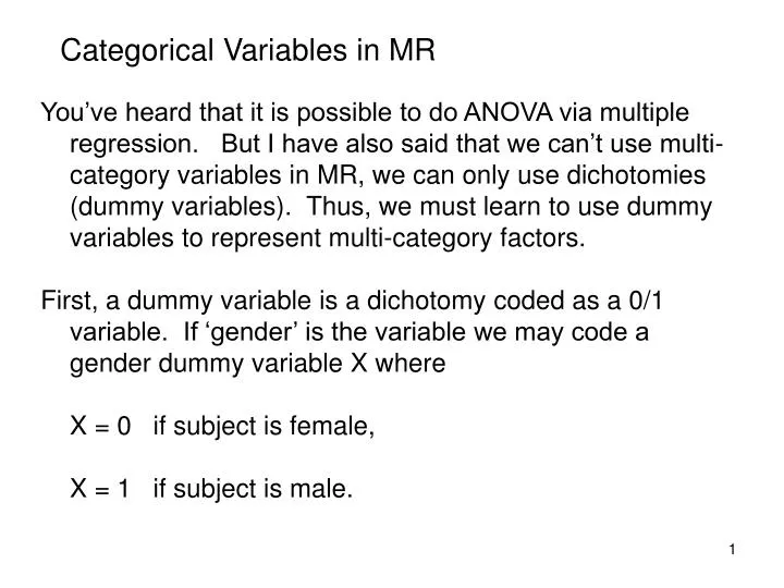
Categorical Variables in MR You’ve heard that it is possible to do ANOVA via multiple regression. But I have also said that we can’t use multi-category variables in MR, we can only use dichotomies (dummy variables). Thus, we must learn to use dummy variables to represent multi-category factors. First, a dummy variable is a dichotomy coded as a 0/1 variable. If ‘gender’ is the variable we may code a gender dummy variable X where X = 0 if subject is female, X = 1 if subject is male.
The Concept of the Dummy Variable in MR We have already seen dummy variables used in MR. When we use a dichotomy like X in MR, we get the typical estimated equation We know that b1 represents the predicted change in Yi associated with 1 unit increase in Xi . Normally this one point change can occur anywhere along the scale of X – a change from 50 to 51 or -10 to -9 would cause the same shift or difference in Yi values. But when Xi is a dummy variable and only takes on two values, a difference of one point can only occur when Xi is no longer equal to 0 and is equal to 1, e.g., when Xi = 0, the subject is female, but when Xi = 1, the subject is male.
The Concept of the Dummy Variable in MR So, the slope b1 for our bivariate regression where X is a dummy variable equals the mean difference between the two represented groups – for this X (gender) the slope b1 is the difference between the means of males and females. Also we can see that will equal b0 when Xi = 0. So the intercept represents the mean for all cases with Xi = 0 (i.e., the mean of Y for the females). We can actually prove this is true if we do some algebra with the formula for b1 where the X’s are all 0s and 1s.
The Concept of the Dummy Variable in MR But it is easier to see this empirically by running descriptive statistics and a t test on two groups, and then running a regression using a dummy variable that represents the 2 groups as our X. This was seen in our output for prinlead with the private vs public variable (private) as our predictor. Recall that the slope was b1 = 2.96 (with t = 4.754) and when we did the t test we obtained the results below.
The Concept of the Dummy Variable in MR Be careful though -- the above results only hold exactly for a dummy variable coded 0/1. For instance, if we have a dichotomy that is coded 1/2 the slope will equal the mean difference (because there is still a one-point difference between the groups), but the intercept will NOT equal the mean for either group. If the dichotomy is coded with numbers that are not one unit apart, then the slope will not equal the mean difference. You can check this by running a regression using a dummy variable that represents the 2 groups with numbers other than 0 and 1.
Dummy Variables to Represent k Groups Suppose now we have 3 groups, say, our familiar ‘practice type’ factor. Until now we have coded this using: T = 1 if subject does physical practice, T = 2 if subject does mental practice, and T = 3 if subject does not practice (ctrl). However, MR will treat T as if it were a number, not a label. Is mental practice (T = 2) “twice” as good/bad or different as physical practice (T = 1)? If not, using X in MR would be a mistake. So we need to represent the 3 groups in some other way. We will use (k-1) dummy variables to represent k groups.
Dummy Variables for k Groups We will use dummy (0/1) variables to differentiate these 3 groups. Let X1 represent ‘Does the subject use physical practice?’ (1 = Yes) and X2 represent ‘Does the subject use mental practice?’ (1 = Yes). If we have one subject from each group, their values of the original factor (T) and the two dummy variables X1 and X2 would be Subject Group T X1 X2 Jim Physical 1 1 0 John Mental 2 0 1 Joe Control 3 0 0
Dummy Variables for k Groups Again here are the scores: X1,X2 Subject Group T X1 X2 Pair Jim Physical 1 1 0 1,0 John Mental 2 0 1 0,1 Joe Control 3 0 0 0,0 We do not need a third variable (X3) that represents ‘Does subject not practice?’ or equivalently ‘Is the subject in the control group?’ (1 = Yes). The pair of values (X1 , X2) is different for each group of subjects so we can tell 3 groups apart using 2 dummy variables.
Dummy Variables for k Groups Suppose we did make that third variable. We’d have Subject Group T X1 X2 X3 X1 +X2 1 - (X1 +X2 )=X3 Jim Phys 1 1 0 0 1 0 John Ment 2 0 1 0 1 0 Joe Ctrl 3 0 0 1 0 1 But notice, X3 is a function of X1 and X2. The formula is X3 = 1 – (X1 + X2 ). Because the variables X1 and X2 completely determine X3 , X3 is redundant. Worse yet, if we try to use X1, X2 and X3 in a regression, MR will not run at all because the three are totally multicollinear! So we can only use any pair of the variables X1, X2 and X3.
(k – 1) Dummy Variables in MR Also note, we interpret b1 as the difference between physical-practice subjects and all others, holding X2 constant. For any one subject, X2 will be constant, but the change in X2 tells us which of the other two groups a subject is in. For all the physical-practice subjects, X2 = 0. For the others, X2 = 0 if they are control s’s (and X1 = 0) or X2 = 1 if they are using mental practice (and X1 = 0). Because of the way we created X1 and X2, we will never have a case where both X1 = 1 and X2 = 1.
(k-1) Dummy Variables in MR Suppose now that we use the variables X1 and X2 in MR. Our estimated regression equation will be = b0 + b1 X1i + b2 X2i The slope b1 represents predicted change in Y for 1 unit increase in X1, holding X2 constant. It is also the difference between the physical-practice group mean and the mean for all other groups combined. The slope b2 represents predicted change in Y for 1 unit increase in X2, holding X1 constant, and it is the mean difference between the mental-practice s's and all others.
(k-1) Dummy Variables in MR Finally in our estimated regression equation = b0 + b1 X1i + b2 X2i the value of b0 is the mean (or predicted score) for the control group, and is the predicted value of Y when the values of all the X's are zero. In a case such as this we might actually be interested in testing whether b0 = 0 because b0 represents the population mean of the control group. So, with the intercept and two slopes we can compute all of the group means.
(k – 1) Dummy Variables in MR Specifically we can see that = bo = for control group = bo + b1 = for physical practice group = bo + b2 = for mental practice group None of our cases ever has because no one ever uses both physical and mental practice together.
Interactions in MR Now that we have seen that we can use dummy variables in MR to represent groups, we will tackle another idea. Suppose we are examining a regression model with a dummy variable and we expect that X relates to Y differently in our 2 groups. Say we are studying the prediction of locus of control (LOC) scores for males and females, and we believe locus of control relates differently to parental control for boys and girls. We can say that there is an interaction of gender and parental control with respect to the locus of control outcome.
Detecting an Interaction How can we tell if we need to be concerned about an interaction like this? One way is to let SPSS help us find it by using the scatter plot. Another is to examine the correlations or slopes. Pull down the Graph menu and make a scatterplot where Y is the variable (f1locus2) and X is f1ctrl2 (parental control). Before you click “OK”, move the variate f1sex into the “Set Markers by” box. This forces SPSS to use different symbols for boys and girls and enables us to edit (double-click) the plot then use ‘Chart Options’ to plot separate regressions for boys and girls.
Detecting an Interaction Here we first see the plot without markers – the relationship looks weak. Then we add the markers by sex and plot two lines. The lines are different, but not dramatically so. It is safe to say the slopes of the two lines are not identical.
Modeling Interactions in MR One solution when we see an interaction is to run separate regression analyses for the groups involved (e.g., boys and girls). To do this we must split the file and run a model with only the predictor variable in it. However, there are drawbacks to this. First of all our sample size for the regressions will be much smaller because we will do two analyses, on parts of the data. Also we will end up with separate slopes and need to do computations by hand to test whether the slopes differ by gender. But as an exercise we will run these two models anyway and compare them to the other approach to see how they relate.
Modeling Interactions in MR The separate models for boys (left) and girls are:
Modeling Interactions in MR The estimated regression models are For boys: And for girls: = .165 -.002 f1ctrl2 = -.179 -.013 f1ctrl2 If we run the same model for all subjects together, we get = -.02 -.006 f1ctrl2
Modeling Interactions in MR With the above approach we run separate regressions for the groups involved if we see a potential interaction. However, a more parsimonious solution would be to model the two slopes via an interaction in a single regression model. Also this approach gives us a test of the interaction (i.e., the difference between the slopes). To do this we need to compute an interaction variable. Suppose X1 is a gender dummy variable and X2 is f1ctrl2 is Xα. Then we can compute the product X3 = X1 X2 = sexdummy f1ctrl2. This new variable takes on values as follows: X3 = 0 if the subject is female X3 = f1ctrl2 = X2 if the subject is male.
Modeling Interactions in MR For the more elegant solution we run a regression that includes X1 (the dummy for gender), X2 (the continuous predictor f1ctrl2), and X3 (the interaction) so our model is Yi = o + 1 X1i + 2 X2i + 3 X3i + ei 1 represents the boy-girl mean difference (or here intercept difference), controlling for X2 and X3, 2 represents the slope of the predictor f1ctrl2, controlling for X1 (gender differences) and X3 (the interaction), and 3 is the interaction, or the sex difference in the f1ctrl2 slope, controlling for X1 and X2.
Modeling Interactions in MR Because X1 is a dummy variable and also because X3 takes on the value 0 for girls, the girls and boys have different models that we can determine even without running SPSS to estimate the model. Since girls have the value 0 for X1 and X3, those variables do not appear in the model for girls. The girls' model is Yi = o + 1 X1i + 2 X2i + 3 X3i + ei = o + 2 X2i + ei , For the boys X1 = 1 and X3 = X2. Thus the boys' model is Yi = o + 1 X1i + 2 X2i + 3 X2i + ei = (o + 1) + (2 + 3 ) X2i + ei
Checking on the Interaction From this output we can see that the girls' estimated regression line is = -.179 -.013 f1ctrl2. This is the same result that appears on slide 19. Also we can compute the boys' model. Their intercept is: b0 + b1 = -.179 + .344 = .165 and the slope (b2 + b3) = -.013 + .011 = -.002. On page 19 the boy's model was .165 -.002 f1ctrl2.
Checking on the Interaction SPSS also then tells us whether the interaction is significant because the test of H0 : 3 = 0 is an interaction test. In this output we see that X3 = sexdummy * f1ctrl2 does not have a significant slope. So even though the lines look different, they are not different enough for us to need to keep the interaction variable X3 in the model.
Adjusted R2 Until now we have only used R2 = SS Regression/ SSTotal as one index of “variance explained”. However, we have heard that R2 can increase even if we add predictors like “the kitchen sink” (all kinds of minimally useful Xs). So because R2 is sensitive to sample size and the number of Xs used, we will learn how “adjusted R2 ” works. The formula is R2 adjusted = We can think of (1 - R2) as the proportion of variance “not accounted for” by our Xs. The number (n-1)/(n-p-1) is the ratio of total df to error df. It is always larger than 1, and gets increasingly larger as we add more predictors.
Adjusted R2 Consider a case with 30 subjects and R2 = .50 for one X (p = 1), but with R2 = .60 with p = 10 predictors. It looks like adding more Xs helped us, but what if many of the added 9 variables are not too useful? Here are the adjusted R2 values R2 = .5, n = 30, p = 1 R2 = .6, n = 30, p = 10 R2 adj =1 – (.50) (29/28) R2 adj = 1 – (.40) (29/19) R2 adj = .48 R2 adj = .39 Once we adjust for throwing in a pile of not-too-useful Xs we see we have effectively explained less than with one X! So unless our additional 9 Xs really add considerably to the model we won’t get a larger adjusted R2.
Tests of Change in R2 (Do more Xs explain more?) Often we will want to know whether adding one X or a set of Xs has significantly increased the explanatory power of our model. We can do this approximately by comparing R2 values, or we can do an exact test of whether R2 has increased in the population. However, for the test to be legitimate the smaller set of Xs must be a subset of those in the larger model. So we can compare these models prinlead = f (tchhappy, f1ses) vs prinlead = f (tchhappy, f1ses, tchinfl). But we can’t compare these: prinlead = f (tchhappy, f1ses) vs prinlead = f (tchhappy, tchinfl, tchangst).
Notation for Increment to R2 Test Let us call the model with more Xs (say pL) the larger model and its R2 will be R2L. Then the model based on a subset of those X’s will be the smaller model with ps predictors and R2s. To test whether the large model has a signifcantly larger explained variance than the small one we test: H0: - = 0 or H0: pS+1 = … pL = 0 We use an F test, called the “Increment to R2” or "change in R2 test to examine these hypotheses.
Notation for Increment to R2 Test Here is the formula for the F test. (R2L - R2s) / (pL – ps) F = (1- R2L) / (n – pL – 1) Notice that (pL – ps) is the number of predictors we have added to the smaller model in an effort to explain more variance in Y. As noted above, we are also asking whether any of the added Xs has a nonzero slope. If all the Xs have slopes equal 0, they have not added anything to our model.
R2 Tests We first begin by noticing that the overall F test in MR is also a test of We can write R2 /p [SSReg/SST] / p F = (1- R2) / (n - p -1) = [SSResidual/SST]/(n – p – 1) However, this is a test based on one R2, so we can say H0: 1 = 2 = … = p = 0 and H0: = 0 are equivalent hypotheses. However, we want to test for a difference or increase in R2 values.
Example of Increment to R2 Test Suppose we want to see whether the three variables to our model for prinlead in the NELS school data set. Our larger model has pL = 4 predictors (tchhappy, tchcomm, tchinfl, and f1ses). Recall that the R2 for the model with 4 Xs is R2L = .368. Our smaller model will be the one with only tchcomm (ps – 1). The smaller R2 will be R2s = .327. So (R2L - R2s ) / (pL – ps)(.368 - .328)/3) =. .040/3 = 20.19 F = (1 - R2L) / (n - pL- 1) = (1 - .368)/ 957 .632/957 This is an F test with (pL – ps) = 3 and (n – pL – 1) = 957 degrees of freedom. It is significant.
Venn Diagrams for R2 Values • If you think back to your primary school math classes many of you will recall encountering • Venn diagrams • Venn diagrams are often used to show intersections and unions of sets and subsets in mathematics, and are typically drawn as overlapping circles or ovals: • The hatched section • where the two circles • overlap represents the • intersection of two sets.
Venn Diagrams for R2 Values We use Venn diagrams in MR to show how much of the variance in our outcome Y we are explaining through the use of different predictors (say, X1, X2 and X3.) One circle will represent variation in Y (I will give this circle a solid outline), and the others will be the predictors. Let us first consider only one predictor, X1. In MR we will use the hatched section where the two circles overlap to represent the common variance X1 Y between the two variables. The higher the correlation between X1 and Y, the more the circles will overlap.
Venn Diagrams for R2 Values Since R2(X, Y) represents the proportion of variance in common between the two variables X and Y if we are willing to consider the total area of the circle for Y to equal 1, then the area where the circles overlap equals R2(X, Y). It is difficult to draw the hatched section to be exactly equal to the proper proportion of the area of Y without special software. So just do a decent job and that will be sufficient. The higher the correlation between X1 and Y, the more X1 Y the circles should overlap. .15 Perhaps here the R2(X1, Y) is about .15.
Venn Diagrams for R2 Values When we have several predictors we need to also consider the degree to which the Xs are intercorrelated when we draw the Venn diagrams. The ideal situation would be one where the circles for the Xs cover a great deal of the area of the circle for Y but do not overlap with each other. Here is such a diagram. I am leaving out the hatching but labeling the overlapping areas instead. Here the total R2 for a regression model of Y on X1, X2 and X3 would be the sum of the areas a + b + c. Also since none of the circles for X1, X2 and X3 overlap, they are all independent. X2 b c X3 a X1 Y
Venn Diagrams for R2 Values Also in this diagram since X1, X2 and X3 are independent, we know that R2(Y, ) = a + b + c = R2(Y, X1 ) + R2(Y, X2 ) + R2(Y, X3 ) However in most cases where the X's are intercorrelated the computation of R2(Y, ), etc., for these diagrams is a bit more complex. So we will see how to compute the values for other cases. X2 b c X3 a X1 Y
Venn Diagrams for R2 Values Let us consider a diagram with two predictors plus Y. As before we will use R2 to represent the proportion of variance in common between two variables, but now we need to worry about the shared variance among the Xs. We need values of R2(X1, X2), R2(Y, X1), R2(Y, X2) and R2(Y; X1, X2) = R2(Y, ). Note that according to the diagram, R2(Y, ) = a + b + c R2(Y, X1 ) = a + c R2(Y, X2 ) = b + c R2(X1, X2) = c + d Y a X1 c b d X2
Venn Diagrams for R2 Values We will run SPSS to get the values of R2(X1, X2), R2(Y, X1), R2(Y, X2) and R2(Y; X1, X2) = R2(Y, ). This will require us to run four regression models. This is easier than using correlations and squaring them, and is necessary when we have two or more predictors (unless we save predicted values which can get very tedious). Suppose we are examining the NELS student data with Y = student morale (f1stumor) X1 = locus of control (f1locus2) and X2 = socioeconomic status (f1ses)
Venn Diagrams for R2 Values Y = student morale (f1stumor) X1 = locus of control (f1locus2) X2 = socioeconomic status (f1ses) R2(Y; locus & ses) = a + b + c = .223 R2(Y, locus [X1]) = a + c = .206 R2(Y, ses [X2]) = b + c = .039 R2(X1, X2) = c + d = .023 We will now get the components by subtraction. Y a X1 c b d X2
Venn Diagrams for R2 Values R2(Y; locus & ses) = a + b + c = .223 R2(Y, locus [X1]) = a + c = .206 R2(Y, ses [X2]) = b + c = .039 R2(X1, X2) = c + d = .023 We use the four quantities and subtract to get components. Area a. This is the amount explained by X1 (locus) only: a = R2(Y; locus & ses) - R2(Y, ses [X2]) a = (a + b + c) - (b + c) a = .223 - .039 = .184 Area b. The amount explained by X2 (ses) only: b = R2(Y; locus & ses) - R2(Y, locus [X1]) b = (a + b + c) - (a + c) b = .223 - .206 = .017 X1 a Y c b d X2
Venn Diagrams for R2 Values R2(Y; locus & ses) = a + b + c = .223 R2(Y, locus [X1]) = a + c = .206 R2(Y, ses [X2]) = b + c = .039 R2(X1, X2) = c + d = .023 There are several ways to get components c and d. Area c. This is the amount explained by both X1 and X2: c = R2(Y; locus & ses) - a - b ) OR R2(Y, ses [X2]) - b c = (a + b + c) - a - b OR (b + c) - b c = .223 - .184 - .017 = .039 - .017 = .022 Area d. The variance shared by X1 and X2 but not common to Y: d = R2(locus; ses) - c = (c + d) - c d = .023 - .022 = .001 X1 Y .184 c d .017 X2
Venn Diagrams for R2 Values Here are all the areas: Area a. The amount explained by X1 (locus) only = .184 Area b. The amount explained by X2 (ses) only= .017 Area c. The amount explained by both X1 and X2= .022 Area d. The variance shared by X1 and X2 but not common to Y = .001 R2(Y; locus & ses) = a + b + c = .223 R2(Y, locus [X1]) = a + c = .206 R2(Y, ses [X2]) = b + c = .039 R2(X1, X2) = c + d = .023 X1 Y .184 .022 .017 .001 X2
Venn Diagrams for R2 Values Lest you think this is some ridiculous exercise I have created simply to torture you, next we will see how this kind of diagram is used in practice -- specifically in an article by Leonie J. Rennie and Keith F. Punch appearing in the Journal of Research Science Teaching (1991, JRST, 28(2), 193-209). They examined the prediction of science achievement from science affect (e.g., liking of science) and prior achievement. Also they examined science achievement at two time points (March and October) for two schools that they refer to as Red School and Blue School.
This R2 shows much common variance. This slide shows the results for achievement and affect in one of two schools. 39% of variance in science achievement was explained by prior achvt and affect.
Slightly less was explained in the second school, but here affect and prior achvt were more independent. This R2 is much smaller.
Later in the year in Red School, even more variance was explained.
Later in the year in the second school, things changed quite a bit in Blue School!