Welcome to Elementary Statistics

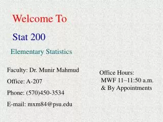
1. Welcome to Elementary Statistics • Statistics is a ‘do’ field. In order to learn, it you must ‘do’ it. • We depend on the TI-83/84 to eliminate the drudgery of calculations. • This is a collaborative class • Hints for success in this class • Work on class topics every day • Form a study group • Don’t get discouraged • As you solve problems, ask yourself “Does this answer make sense?’ • Get help as soon as you need it • From me • Tutorial Center • Don’t get behind

2. What’s the point? • Surrounded by examples • crime, sports, politics • Interpret data to make decisions • Analyze information • Survey results and your critical eye • Do samples represent population • Is sample big enough? • How was sample chosen? What ‘type’ of people/things selected? • Are survey questions loaded? • Are graphs properly displayed, data complete, context stated? • Was there anything ‘confounding’ the results?

3. Math 10 - Elementary Statistics Text: Collaborative Statisticsby Susan Dean and Barbara Illowsky Available online as a free download.

4. Chapter 1 Sampling and Data

5. Chapter 1 Objectives The Student will be able to • Define, in context, key statistical terms. • Define, in context, and identify different sampling techniques. • Understand the variability of data. • Create and interpret Relative Frequency Tables.

6. Some definitions • Statistics • collection, analysis, interpretation and presentation of data • descriptive statistics • inferential statistics • Probability • mathematical tool used to study randomness • theoretical • empirical

7. Key terms • Population • entire collection of persons, things or objects under study • Sample • a portion of the larger population • Parameter • number that is a property of the population • Average, standard deviation, proportion (µ, σ, p) • Statistic • number that is a property of the sample • Average, standard deviation, proportion (x-bar, s, p’)

8. Key terms • Variable • the characteristic of interest for each person or thing in a population • numerical • categorical • Data - data type example • the actual values of the variable • qualitative • quantitative • discrete • continuous An ‘in context’ example

9. Sampling • Taking a portion of the total population • Need for random sample • Represent the population (has the same characteristics as population) • each element of the population should have an equal chance of being chosen Population Sample

10. Sampling Methods • Simple random sampling • each member of a population initially has an equal chance of being selected for the sample • Random number generator • With replacement • Without replacement • Stratified sample • divide population into groups and then take a sample from each group • Cluster sample • divide population into groups and then randomly select some of the groups and sample all members of those groups

11. Sampling Methods • Systematic sample • select a starting point and take every nth piece of data from a listing of the population • Convenience sample • using results that are readily available – just happen to be there • Why a problem?

12. Determine the type of sampling used (simple random, stratified, systematic, cluster, or convenience). • A soccer coach selects 6 players from a group of boys aged 8 to 10, 7 players from a group of boys aged 11 to 12, and 3 players from a group of boys aged 13 to 14 to form a recreational soccer team. • A pollster interviews all human resource personnel in five different high tech companies. • An engineering researcher interviews 50 women engineers and 50 men engineers. • A medical researcher interviews every third cancer patient from a list of cancer patients at a local hospital. • A high school counselor uses a computer to generate 50 random numbers and then picks students whose names correspond to the numbers. • A student interviews classmates in his algebra class to determine how many pairs of jeans a student owns, on the average.

13. Example 1.6.1 – Determine whether or not the following samples are representative. If they are not, discuss the reasons. 1. To find the average GPA of all students in a university, use all honor students at the university as the sample. 2. To find out the most popular cereal among young people under the age of 10, stand outside a large supermarket for three hours and speak to every 20th child under the age of 10 who enters the supermarket. 3. To find the average annual income of all adults in the U.S., sample U.S. congresspersons. Create a cluster sample by considering each state as a stratum (group). By using a simple random sampling, select states to be part of the cluster. Then survey every U.S. congressperson in the cluster. 4. To determine the proportion of people taking public transportation to work, survey 20 people in NYC. Conduct the survey by sitting in Central Park on a bench and interviewing every person who sits next to you. 5. To determine the average cost of a two day stay in a hospital in Massachusetts, survey 100 hospitals across the state using simple random sampling.

14. Variation • In data • In samples • The larger the sample the better it represents the population – Law of Large numbers – and sample statistics get closer to population parameters

15. Critical Evaluation • Problems with samples • Self-selected samples • Sample size issues • Undue influence • Non-response or refusal of subject to participate • Causality • Self-funded or Self-interest studies • Misleading Use of Data • Confounding

16. Frequency Table • Data value • Frequency • how many times the data value occurs • Relative Frequency • frequency/(total number of data values) • Cumulative Relative Frequency • summation of previous relative frequencies An example – How many siblings do you have?

17. And, oh, btw • A word on fractions • You DO NOT have to reduce fractions in this course. In fact, I INSIST that you don’t. • If you convert to decimal, take answer to 4 decimal places. • A word on rounding answers • Don’t round until the final answer • In general, the final answer should have one more decimal place than the data used to get the answer • HOWEVER, the rule of thumb for this course will be probabilities (relative frequencies) to 4 decimal places, everything else to 2, unless you are told otherwise.

18. Chapter 2 Descriptive Statistics: Displaying and Measuring Data

19. Chapter 2 Objectives The Student will be able to • Display data graphically and interpret graphs: stemplots, histograms and boxplots. • Recognize, describe, and calculate the measures of location of data: quartiles and percentiles. • Recognize, describe, and calculate the measures of the center of data: mean, median, and mode. • Recognize, describe, and calculate the measures of the spread of data: variance, standard deviation, and range.

20. Measures of the “Center” of the Data • Mean or average • Use calculator • Median - the middle data value • 50% of data below, 50% above • Data MUST be ordered from lowest to highest • Use calculator • Mode - the most frequent data value • Have to count (or put in a frequency table)

21. Measures of Location of Data • Relative to other data values • Quartiles • Splits data into 4 equal groups that contain the same percentage of data • Data must be put in numerical order • Use calculator • Percentiles • Splits data into 100 equal groups • Data must be put in numerical order • Relative to the mean • x = x-bar + zs • z < 0, data value is below the mean • z > 0, data value is above the mean • IQR – interquartile range • IQR = Q3 – Q1 • Middle 50% of data • Determine potential outliers • Data value < Q1 – 1.5(IQR) • Data value > Q3 + 1.5(IQR)

22. Measures of the “Spread” of Data • Range • Difference between high value and low value • Standard deviation • ‘distance’ from the mean • Sample versus population • Variance • Sample s2 • Population 2 Using calcuator

23. Pictures worth a 1000 words • ‘Charts’ • Stem and Leaf Graphs – example • Line Graphs – not using • Bar Graphs – not using • Histograms – Let’s try one • sort data into bars or intervals • 5 to 15 bars • horizontal axes is what the data represents • vertical axes labeled “frequency” or “relative frequency” • Boxplots – Try with histogram data • need min, median, first and second quartile, max

24. Chapter 3 Probability Topics Chapter Objectives

25. Chapter 3 Objectives The student will be able to • Understand and use the terminology of probability. • Calculate probabilities by listing event sample spaces and counting. • Determine whether two events are mutually exclusive or independent. • Calculate probabilities using the Addition Rules and Multiplication Rules. • Construct and interpret Contingency Tables. • Construct and interpret Tree Diagrams.

26. Activity • # of students in class ____ • # with change in pocket or purse ____ • # who have a sister ____ • # who have change and a sister ____ • P(change) = ____ • P(sister) = ____ • P(change and sister) = ____ • P(change|sister) = ____

27. Definitions • Experiment - planned operations carried out under controlled conditions • Chance experiment - results not predetermined • Outcome - result of an experiment • Sample space - set of all possible outcomes • Event - any combination of outcomes • Probability - long-term relative frequency of an outcome, I.E. it is a fraction - a number between 0 and 1, inclusive • OR - as in A OR B - outcome is in A or is in B or is in both A and B • AND - outcome is in both A and B at the same time • Complement - denoted A’ (read “A prime”) - all outcomes that are not in A

28. More Definitions • Conditional Probability of A given B - probability of A is calculated knowing B has already occurred • P(A|B) = P(A and B) ÷ P(B) • Independent events - the chance of event A occurring does not affect the chance of event B occurring and vice versa • must prove one of the following • P(A|B) = P(A) • P(B|A) = P(B) • P(A and B) = P(A)P(B) • Mutually Exclusive - event A and event B cannot occur at the same time, they don’t share outcomes • P(A and B) = 0

29. The Tale of Two Die • Experiment • Toss two die, record value showing on each die • Sample space (S) • {(1,1), (1,2), (1,3), (1,4), (1,5), (1,6), (2,1), (2,2), (2,3), (2,4), (2,5), (2,6), (3,1), (3,2), (3,3), (3,4), (3,5), (3,6), (4,1), (4,2), (4,3), (4,4), (4,5), (4,6), (5,1), (5,2), (5,3), (5,4), (5,5), (5,6), (6,1), (6,2), (6,3), (6,4), (6,5), (6,6)}

30. The Tale of Two Die • Let A = the event the sum of the faces of the die is odd • A = {(1,2), (1,4), (1,6), (2,1), (2,3), (2,5), (3,2), (3,4), (3,6), (4,1), (4,3), (4,5), (5,2), (5,4), (5,6), (6,1), (6,3), (6,5)} • Let B = event of getting a double • B = {(1,1), (2,2), (3,3), (4,4), (5,5), (6,6)} • Let D = event that at least one face is a 2 • D = {(1,2), (2,1), (2,2), (2,3), (2,4), (2,5), (2,6), (3,2), (4,2), (5,2), (6,2)}

31. The Tale of Two Die • P(A) = ___ P(B) = ___ P(D) = ___ • P(D and A) = ____ • P(A and B) = ____ • P(A or D) = ____ • P(D|A) = ____ • P(A|D) = ____

32. What if the sample space is not listed? Need formulas: Addition Rule: P(A OR B) = P(A) + P(B) – P(A AND B) Multiplication Rule: P(A AND B) = P(B)*P(A|B) P(A AND B) = P(A)*P(B|A) Example: P(C) = 0.4, P(D) = 0.5, P(C|D) = 0.6 • P(C and D) = _____ • Are C and D mutually exclusive? • Are C and D independent? • P(C or D) = • P(D|C) =

33. Contingency Tables • A table that displays sample values in relation to two different variables that may be contingent on one another. • Example - Performance on Job vs. performance in training

34. Tree Diagram • A “graph” used to determine outcomes of an experiment • Consists of “branches” that are labeled with either frequencies or probabilities • Once probability (frequency) entered on branches, probability (frequency) can be “read” by multiplying down branches and/or adding across branches

35. Tree Diagram • Experiment - cup with 8 black and 3 yellow beads. Draw 2 beads , one at a time, with replacement. Record bead color.

36. Review for Exam 1 • What’s fair game • Chapter 1 • Chapter 2 • Chapter 3 • 21 multiple choice questions • The last 3 quarters exams • What to bring with you • Scantron (#2052), pencil, eraser, calculator, 1 sheet of notes (8.5x11 inches, both sides)