Linearization of Interacting Tank-in-Series System Using MATLAB Simulink
This homework assignment involves linearizing the interacting tank-in-series system at a specified operating point derived from previous parameter values. You will need to utilize MATLAB Simulink to model the system, incorporating your specific flow rate from your Student ID. The assignment requires submission of both the mdl-file and screenshots of the Simulink model and simulation results. Ensure that you perform the linearization accurately around the operating point with the provided steady-state conditions to achieve the desired model outputs.

Linearization of Interacting Tank-in-Series System Using MATLAB Simulink
E N D
Presentation Transcript
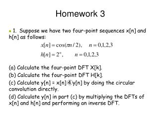
Chapter 2 Linearization Homework 3 Linearize the the interacting tank-in-series system for the operating point resulted by the parameter values as given in Homework 2. • For qi, use the last digit of your Student ID. For example: Kartika qi= 8 liters/s. • Submit the mdl-file and the screenshots of the Matlab-Simulink file + scope. qi h1 h2 q1 a1 a2 v1 v2
Chapter 2 Linearization Solution to Homework 3 • The model of the system is: • As can be seen from the result of Homework 2, the steady state parameter values, which are taken to be the operating point, are:
Chapter 2 Linearization Solution to Homework 3 • The linearization around the operating point (h1,0,h2,0,qi,0) is performed as follows:
Chapter 2 Linearization Solution to Homework 3
Chapter 2 Linearization Solution to Homework 3
Chapter 2 Linearization Solution to Homework 3
Chapter 2 Linearization Solution to Homework 3
Chapter 2 Linearization Solution to Homework 3 : h1, original model : h2, original model : h1, linearized model : h2, linearized model
Chapter 2 Linearization Solution to Homework 3 : h1, original model : h2, original model : h1, linearized model : h2, linearized model
Chapter 2 Linearization Solution to Homework 3 : h1, original model : h2, original model : h1, linearized model : h2, linearized model
System Modeling and Identification Chapter 3 Analysis of Process Models
Chapter 3 Analysis of Process Models State Space Process Models • Consider a continuous-time MIMO system with m input variables and r output variables. The relation between input and output variables can be expressed as: : vector of state space variables : vector of input variables : vector of output variables
Chapter 3 State Space Process Models Solution of State Space Equations • Consider the state space equations: • Taking the Laplace Transform yields:
Chapter 3 State Space Process Models Solution of State Space Equations • After the inverse Laplace transformation, • The solution of state space equations depends on the roots of the characteristic equation:
Chapter 3 State Space Process Models Solution of State Space Equations Consider a matrix . Calculate .
Chapter 3 State Space Process Models Canonical Transformation • Eigenvalues of A, λ1, …, λn are given as solutions of the equation det(A–λI) = 0. • If the eigenvalues of A are distinct, then a nonsingular matrix T exists, such that: is a diagonal matrix of the form
Chapter 3 State Space Process Models Canonical Transformation • Example Perform the canonical transformation to the state space equations below • The eigenvalues of A
Chapter 3 State Space Process Models Canonical Transformation • The eigenvectors of A
Chapter 3 State Space Process Models Canonical Transformation ~ The equivalence transformation can now be done, with x = Tx. Then, the state space equations As the result, we obtain a state space in canonical form,
Chapter 3 Homework 4 State Space Process Models • Make yourself familiar with the canonical transformation. Obtain the canonical form of the state space below.
Chapter 3 Homework 4 (New) State Space Process Models • Perform the canonical transformation for the following state space equation. NEW • Hint: Learn the following functions in Matlab: [V,D] = eig(X)