Download
1 / 69
730 likes | 1.04k Views
Reinforcement Learning (RL). Learning from rewards (and punishments) Learning to assess the value of states. Learning goal directed behavior. RL has been developed rather independently from two different fields: Dynamic Programming and Machine Learning (Bellman Equation).

E N D
Reinforcement Learning (RL) Learning from rewards (and punishments) Learning to assess the value of states. Learning goal directed behavior. • RL has been developed rather independently from two different fields: • Dynamic Programming and Machine Learning (Bellman Equation). • Psychology (Classical Conditioning) and later Neuroscience (Dopamine System in the brain)
Back to Classical Conditioning U(C)S = Unconditioned Stimulus U(C)R = Unconditioned Response CS = Conditioned Stimulus CR = Conditioned Response I. Pawlow
Less “classical” but also Conditioning ! (Example from a car advertisement) Learning the association CS → U(C)R Porsche → Good Feeling
Why would we want to go back to CC at all?? So far: We had treated Temporal Sequence Learning in time- continuous systems (ISO, ICO, etc.) Now: We will treat this in time-discrete systems. ISO/ICO so far did NOT allow us to learn: GOAL DIRECTED BEHAVIOR ISO/ICO performed: DISTURBANCE COMPENSATION (Homeostasis Learning) The new RL= formalism to be introduced now will indeed allow us to reach a goal: LEARNING BY EXPERIENCE TO REACH A GOAL
Overview over different methods – Reinforcement Learning You are here !
Overview over different methods – Reinforcement Learning And later also here !
Notation US = r,R = “Reward” (similar to X0 in ISO/ICO) CS = s,u = Stimulus = “State1” (similar to X1 in ISO/ICO) CR = v,V = (Strength of the) Expected Reward = “Value” UR = --- (not required in mathematical formalisms of RL) Weight = w = weight used for calculating the value; e.g. v=wu Action = a = “Action” Policy = p = “Policy” “…” = Notation from Sutton & Barto 1998, red from S&B as well as from Dayan and Abbott. 1 Note: The notion of a “state” really only makes sense as soon as there is more than one state.
A note on “Value” and “Reward Expectation” If you are at a certain state then you would value this state according to how much reward you can expect when moving on from this state to the end-point of your trial. Hence: Value = Expected Reward ! More accurately: Value = Expected cumulative future discounted reward. (for this, see later!)
Types of Rules • Rescorla-Wagner Rule: Allows for explaining several types of conditioning experiments. • TD-rule (TD-algorithm) allows measuring the value of states and allows accumulating rewards. Thereby it generalizes the Resc.-Wagner rule. • TD-algorithm can be extended to allow measuring the value of actions and thereby control behavior either by ways of • Q or SARSA learning or with • Actor-Critic Architectures
Overview over different methods – Reinforcement Learning You are here !
Rescorla-Wagner Rule Pre-Train Train Result Pavlovian: Extinction: Partial: u→r u→v=max u→r u→● u→v=0 u→r u→● u→v<max We define: v = wu, with u=1 or u=0, binary and w→w + mdu with d = r - v The associability between stimulus u and reward r is represented by the learning rate m. This learning rule minimizes the avg. squared error between actual reward r and the prediction v, hence min<(r-v)2> We realize that d is the prediction error.
Pawlovian Extinction Partial Stimulus u is paired with r=1 in 100% of the discrete “epochs” for Pawlovian and in 50% of the cases for Partial.
Pre-Train Train Result Blocking: u1→r u1+u2→r u1→v=max, u2→v=0 For Blocking: The association formed during pre-training leads to d=0. As w2 starts with zero the expected reward v=w1u1+w2u2 remains at r. This keeps d=0 and the new association with u2 cannot be learned. Rescorla-Wagner Rule, Vector Form for Multiple Stimuli We define: v = w.u, and w→w + mdu with d = r – v Where we use stochastic gradient descent for minimizing d Do you see the similarity of this rule with the d-rule discussed earlier !?
Rescorla-Wagner Rule, Vector Form for Multiple Stimuli Pre-Train Train Result Inhibitory: u1+u2→●, u1→r u1→v=max, u2→v<0 Inhibitory Conditioning: Presentation of one stimulus together with the reward and alternating presenting a pair of stimuli where the reward is missing. In this case the second stimulus actually predicts the ABSENCE of the reward (negative v). Trials in which the first stimulus is presented together with the reward lead to w1>0. In trials where both stimuli are present the net prediction will be v=w1u1+w2u2 = 0. As u1,2=1 (or zero) and w1>0, we get w2<0 and, consequentially, v(u2)<0.
Rescorla-Wagner Rule, Vector Form for Multiple Stimuli Pre-Train Train Result Overshadow: u1+u2→r u1→v<max, u2→v<max Overshadowing: Presenting always two stimuli together with the reward will lead to a “sharing” of the reward prediction between them. We get v= w1u1+w2u2 = r. Using different learning rates m will lead to differently strong growth of w1,2 and represents the often observed different saliency of the two stimuli.
Rescorla-Wagner Rule, Vector Form for Multiple Stimuli Pre-Train Train Result Secondary: u1→r u2→u1 u2→v=max Secondary Conditioning reflect the “replacement” of one stimulus by a new one for the prediction of a reward. As we have seen the Rescorla-Wagner Rule is very simple but still able to represent many of the basic findings of diverse conditioning experiments. Secondary conditioning, however, CANNOT be captured. (sidenote: The ISO/ICO rule can do this!)
Predicting Future Reward The Rescorla-Wagner Rule cannot deal with the sequentiallity of stimuli (required to deal with Secondary Conditioning). As a consequence it treats this case similar to Inhibitory Conditioning lead to negative w2. Animals can predict to some degree such sequences and form the correct associations. For this we need algorithms that keep track of time. Here we do this by ways of states that are subsequently visited and evaluated. Sidenote: ISO/ICO treat time in a fully continuous way, typical RL formalisms (which will come now) treat time in discrete steps.
Prediction and Control • The goal of RL is two-fold: • To predict the value of states (exploring the state space following a policy) – Prediction Problem. • Change the policy towards finding the optimal policy – Control Problem. Terminology (again): • State, • Action, • Reward, • Value, • Policy
Markov Decision Problems (MDPs) rewards actions states If the future of the system depends always only on the current state and action then the system is said to be “Markovian”.
What does an RL-agent do ? An RL-agent explores the state space trying to accumulate as much reward as possible. It follows a behavioral policy performing actions (which usually will lead the agent from one state to the next). For the Prediction Problem: It updates the value of each given state by assessing how much future (!) reward can be obtained when moving onwards from this state (State Space). It does not change the policy, rather it evaluates it. (Policy Evaluation).
For the Control Problem: It updates the value of each given action at a given state and of by assessing how much future reward can be obtained when performing this action at that state (State-Action Space, which is larger than the State Space). and all following actions at the following state moving onwards. Guess: Will we have to evaluate ALL states and actions onwards?
What does an RL-agent do ? Exploration – Exploitation Dilemma: The agent wants to get as much cumulative reward (also often called return) as possible. For this it should always perform the most rewarding action “exploiting” its (learned) knowledge of the state space. This way it might however miss an action which leads (a bit further on) to a much more rewarding path. Hence the agent must also “explore” into unknown parts of the state space. The agent must, thus, balance its policy to include exploitation and exploration. Policies • Greedy Policy: The agent always exploits and selects the most rewarding action. This is sub-optimal as the agent never finds better new paths.
Policies where Qa is value of the currently to be evaluated action a and T is a temperature parameter. For large T all actions have approx. equal probability to get selected. • e-Greedy Policy: With a small probability e the agent will choose a non-optimal action. *All non-optimal actions are chosen with equal probability.* This can take very long as it is not known how big e should be. One can also “anneal” the system by gradually lowering e to become more and more greedy. • Softmax Policy:e-greedy can be problematic because of (*). Softmax ranks the actions according to their values and chooses roughly following the ranking using for example:
Overview over different methods – Reinforcement Learning You are here !
Towards TD-learning – Pictorial View In the following slides we will treat “Policy evaluation”: We define some given policy and want to evaluate the state space. We are at the moment still not interested in evaluating actions or in improving policies. Back to the question: To get the value of a given state, will we have to evaluate ALL states and actions onwards? There is no unique answer to this! Different methods exist which assign the value of a state by using differently many (weighted) values of subsequent states. We will discuss a few but concentrate on the most commonly used TD-algorithm(s). Temporal Difference (TD) Learning
Lets, for example, evaluate just state 4: Tree backup methods: Most simplistically and very slow: Exhaustive Search: Update of state 4 takes all direct target states and all secondary, ternary, etc. states into account until reaching the terminal states and weights all of them with their corresponding action probabilities. Mostly of historical and theoretical relevance: Dynamic Programming: Update of state 4 takes all direct target states (9,10,11) into account and weights their rewards with the probabilities of their triggering actions p(a5), p(a7), p(a9).
Linear backup methods Full linear backup: Monte Carlo [= TD(1)]:Sequence C (4,10,13,15): Update of state 4 (and 10 and 13) can commence as soon as terminal state 15 is reached.
Linear backup methods Single step linear backup: TD(0):Sequence A:(4,10) Update of state 4 can commence as soon as state 10 is reached. This is the most important algorithm.
Linear backup methods Weighted linear backup: TD(l): Sequences A, B, C: Update of state 4 uses a weighted average of all linear sequences until terminal state 15.
For the following: Note: RL has been developed largely in the context of machine learning. Hence all mathematically rigorous formalisms for RL comes from this field. A rigorous transfer to neuronal model is a more recent development. Thus, in the following we will use the machine learning formalism to derive the math and in parts relate this to neuronal models later. This difference is visible from using STATES st for the machine learningformalism and TIME t when talking about neurons. Why are we calling these methods “backups” ? Because we move to one or more next states, take their rewards&values, and then move back to the state which we would like to update and do so!
Formalising RL: Policy Evaluation with goal to find the optimal value function of the state space We consider a sequence st, rt+1, st+1, rt+2, . . . , rT , sT . Note, rewards occur downstream (in the future) from a visited state. Thus, rt+1 is the next future reward which can be reached starting from state st. The complete return Rt to be expected in the future from state st is, thus, given by: where g≤1 is a discount factor. This accounts for the fact that rewards in the far future should be valued less. Reinforcement learning assumes that the value of a state V(s) is directly equivalent to the expected return Ep at this state, where p denotes the (here unspecified) action policy to be followed. Thus, the value of state st can be iteratively updated with:
This is why it is called TD (temp. diff.) Learning We use a as a step-size parameter, which is not of great importance here, though, and can be held constant. Note, if V(st) correctly predicts the expected complete return Rt, the update will be zero and we have found the final value. This method is called constant-aMonte Carlo update. It requires to wait until a sequence has reached its terminal state (see some slides before!) before the update can commence. For long sequences this may be problematic. Thus, one should try to use an incremental procedure instead. We define a different update rule with: The elegant trick is to assume that, if the process converges, the value of the next state V(st+1) should be an accurate estimate of the expected return downstream to this state (i.e., downstream to st+1). Thus, we would hope that the following holds: Indeed, proofs exist that under certain boundary conditions this procedure, known as TD(0), converges to the optimal value function for all states.
In principle the same procedure can be applied all the way downstream writing: Thus, we could update the value of state st by moving downstream to some future state st+n−1 accumulating all rewards along the way including the last future reward rt+n and then approximating the missing bit until the terminal state by the estimated value of state st+n given as V(st+n). Furthermore, we can even take different such update rules and average their results in the following way: where 0≤l≤1. This is the most general formalism for a TD-rule known as forward TD(l)-algorithm, where we assume an infinitely long sequence.
Linear backup methods Weighted linear backup: TD(l): Sequences A, B, C: Update of state 4 uses a weighted average of all linear sequences until terminal state 15.
The disadvantage of this formalism is still that, for all l > 0, we have to wait until we have reached the terminal state until update of the value of state st can commence. There is a way to overcome this problem by introducing eligibility traces(Compare to ISO/ICO before!). Let us assume that we came from state A and now we are currently visiting state B. B’s value can be updated by the TD(0) rule after we have moved on by only a single step to, say, state C. We define the incremental update as before as: Normally we would only assign a new value to state B by performing V(sB) ← V(sB) + adB, not considering any other previously visited states. In using eligibility traces we do something different and assign new values to all previously visited states, making sure that changes at states long in the past are much smaller than those at states visited just recently. To this end we define the eligibility trace of a state as: Thus, the eligibility trace of the currently visited state is incremented by one, while the eligibility traces of all other states decay with a factor of gl.
In our example we will, thus, also update the value of state A by V(sA) ← V(sA)+ adB xB(A). This means we are using the TD-error dB from the state transition B → C weight it with the currently existing numerical value of the eligibility trace of state A given by xB(A) and use this to correct the value of state A “a little bit”. This procedure requires always only a single newly computed TD-error using the computationally very cheap TD(0)-rule, and all updates can be performed on-line when moving through the state space without having to wait for the terminal state. The whole procedure is known as backward TD(l)-algorithmand it can be shown that it is mathematically equivalent to forward TD(l) described above. Instead of just updating the most recently left state st we will now loop through all states visited in the past of this trial which still have an eligibility trace larger than zero and update them according to: Rigorous proofs exist the TD-learning will always find the optimal value function (can be slow, though).
TD(0) on a 9x9 grid Asymptotic convergence of one weight. Learning Rate 0.004 Learning Rate 0.4 Learning Rate 0.4 and dropping over time.
Reinforcement Learning – Relations to Brain Function I You are here !
We had defined: (first lecture!) Trace u1 How to implement TD in a Neuronal Way Now we have:
v(t+1)-v(t) Note: v(t+1)-v(t) is acausal (future!). Make it “causal” by using delays. Serial-Compound representations X1,…Xn for defining an eligibility trace. How to implement TD in a Neuronal Way
Forward shift because of acausal derivative How does this implementation behave: wi ← wi + mdxi
Observations d-error moves forward from the US to the CS. The reward expectation signal extends forward to the CS.
Reinforcement Learning – Relations to Brain Function II You are here !
TD-learning & Brain Function Omission of reward leads to inhibition as also predicted by the TD-rule. This neuron is supposed to represent the d-error of TD-learning, which has moved forward as expected. DA-responses in the basal ganglia pars compacta of the substantia nigra and the medially adjoining ventral tegmental area (VTA).
TD-learning & Brain Function This is even better visible from the population response of 68 striatal neurons This neuron is supposed to represent the reward expectation signal v. It has extended forward (almost) to the CS (here called Tr) as expected from the TD-rule. Such neurons are found in the striatum, orbitofrontal cortex and amygdala.
TD-learning & Brain Function Deficiencies There are short-latency Dopamine responses! These signals could pro-mote the discovery of agency (i.e. those ini-tially unpredicted events that are caused by the agent) and subsequent identification of critical causative actions to re-select components of behavior and context that immediately pre-cede unpredicted sensory events. When the animal/agent is the cause of an event, re-peated trials should en-able the basal ganglia to converge on behavioral and contextual compo-nents that are critical for eliciting it, leading to the emergence of a novel action. DA Signal leads to the learning of this self-triggered association! =cause-effect Incompatible to a serial compound representation of the stimulus as the d-error should move step by step forward, which is not found. Rather it shrinks at r and grows at the CS.
Reinforcement Learning – The Control Problem So far we have concentrated on evaluating an unchanging policy. Now comes the question of how to actually improve a policy p trying to find the optimal policy. • We will discuss: • Actor-Critic Architectures • SARSA Learning • Q-Learning Abbreviation for policy: p
Reinforcement Learning – Control Problem I You are here !
This is a closed-loop system before learning Control Loops Retraction reflex Bump An old slide from some lectures earlier! Any recollections? ? The Basic Control Structure Schematic diagram of A pure reflex loop
Control Loops A basic feedback–loop controller (Reflex) as in the slide before.