Download
1 / 65
780 likes | 1.68k Views
Part IV TYPES OF GPS OBSERVABLE AND METHODS OF THEIR PROCESSING. GS608. Basic GPS Observables. Pseudoranges precise/protected P1, P2 codes (Y-code under AS) - available only to the military users clear/acquisition C/A code - available to the civilian users

E N D
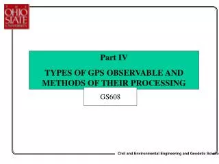
Part IV TYPES OF GPS OBSERVABLE AND METHODS OF THEIR PROCESSING GS608
Basic GPS Observables • Pseudoranges • precise/protected P1, P2 codes (Y-code under AS) • - available only to the military users • clear/acquisition C/A code • - available to the civilian users • Carrier phases • L1, L2 phases, used mainly in geodesy and surveying • Range-rate (Doppler)
Basic GPS Observables • Pseudoranges- geometric range between the transmitter and the receiver, distorted by the lack of synchronization between satellite and receiver clocks, and the propagation media • recovered from the measured time differencebetween the instant of transmission and the epoch of reception. • P-code pseudoranges can be as good as 20 cmor less, while the L1 C/A code range noise level reaches even a meter or more
Basic GPS observables • Carrier phase-a difference between the phases of a carrier signal received from a spacecraft and a reference signal generated by the receiver’s internal oscillator • contains the unknown integer ambiguity, N, i.e., the number of phase cycles at the starting epoch that remains constant as long as the tracking is continuous • phase cycle slipor loss of lockintroduces a new ambiguity unknown. • typical noise of phase measurements is generally of the order of a few millimeters or less
Ambiguity: the initial bias in a carrier-phase observation of an arbitrary number of cycles between the satellite and the receiver; the uncertainty of the number of complete cycles a receiver is attempting to count. • The initial phase measurement made when a GPS receiver first locks onto a satellite signal is ambiguous by an integer number of cycles since the receiver has no way of knowing when the carrier wave left the satellite. • This ambiguity remains constant as long as the receiver remains locked onto the satellite signal and is resolved when the carrier-phase data are processed. • If wavelength is known, the distance to a satellite can be computed once the total number of cycles is established via carrier-phase processing.
Doppler Effect on GPS observable • The Doppler equation for electromagnetic wave, where fr and fs are received and transmitted frequencies • In case of moving emitter or moving receiver the receiver frequency is Doppler shifted • The difference between the receiver and emitted frequencies is proportional to the radial velocity vr of the emitter with respect to the receiver
Doppler Effect on GPS observable • For GPS satellites orbiting with the mean velocity of 3.9 km/s, assuming stationary receiver, neglecting Earth rotation, • the maximum radial velocity 0.9 km/s is at horizon • and is zero at the epoch of closest approach • For 1.5 GHz frequency the Doppler shift is 4.5·103 Hz we get: • 4.5 cycles phase change after 1 millisecond, or change in the range by 90 cm
Phase Observable • Instantaneous circular frequencyf is a derivative of the phase with respect to time • By integrating frequency between two time epochs the signal’s phase results • Assuming constant frequency, setting the initial phase (t0) to zero, and taking into account the signal travel time ttr corresponding to the satellite-receiver distance , we get
Pseudorange Observable tr, ts – time of signal reception at the receiver and the signal transmit at by the satellite (both are subject to time errors, i.e., offsets from the true GPS time) dtr,dts – receiver and transmitter (satellite) clock corrections (errors) c – speed of light e – random errors (white noise) - geometric range to the satellite
Taking into account all error sources (and also simplifying some terms), we arrive at the final observation equations of the following form (for pseudorange and phase observable)
Basic GPS Observable 1/4 and The primary unknowns are Xi, Yi, Zi – coordinates of the user (receiver) 1,2 stand for frequency on L1 and L2, respectively i –denotes the receiver, while k denotes the satellite
i.e., in our earlier notation Basic GPS Observable 2/4 1 19 cm and 2 24 cm are wavelengths of L1 and L2 phases Using our earlier notation for the ionospheric correction we have:
Basic GPS Observables 3/4 dti - the i-th receiver clock error dtk - the k-th transmitter (satellite) clock error f1, f2 - carrier frequencies c - the vacuum speed of light multipath on phases and ranges bi,1,bi,2, bi,3- interchannel bias terms for receiver i that represent the possible time non-synchronization of the four measurements
The above equations are non-linear and require linearization (Taylor series expansion) in order to be solved for the unknown receiver positions and (possibly) for other nuisance unknowns, such as receiver clock correction • Since we normally have more observations than the unknowns, we have a redundancy in the observation system, which must consequently be solved by the Least Squares Adjustment technique • Secondary (nuisance) parameters, or unknowns in the above equations are satellite and clock errors, troposperic and ionospheric errors, multipath, interchannel biases and integer ambiguities. These are usually removed by differential GPS processing or by a proper empirical model (for example troposphere), and processing of a dual frequency signal (ionosphere).
Basic GPS Observable 4/4 • Assume that ionospheric effect is removed from the equation by applying the model provided by the navigation message • Assume that tropospheric effect is removed from the equation by estimating the dry+wet effect based on the tropospheric model (e.g., by Saastamoinen, Goad and Goodman, Chao, Lanyi) • Satellite clock correction is also applied based on the navigation message • Multipath and interchannel bias are neglected • The resulting range equation : Four unknowns: 3 receiver coordinates and receiver clock correction corrected observable
Instantaneous Doppler • Observed Doppler shift scaled to range rate; time derivative of the phase or pseudorange observation equation Instantaneous radial velocity between the satellite j and the receiver i, and v is satellite tangential velocity, see a slide “Doppler effect on GPS observable” (corresponds to in the notation used in figure 6.3)
Instantaneous Doppler • Used primarily to support velocity estimation • Can be used for point positioning • Are instantaneous position vector of the satellite, and the unknown receiver position vector; correspond to rs and rp in the notation used in Figure 6.3 • dot denotes time derivative
Integrated Doppler Observable • The frequency difference between the nominal (sent) signal and the locally generated replica fgcan be used to recover pseudorange difference through so-called integrated Doppler count (more accurate than instantaneous Doppler): • Observed: Njk • Where ikand ij are the distances from the receiver i to the position of the satellite at epochs k and j.
Basic GPS observables(simplified form) R1 = r + cdt +I / f12 + T + eR1 R2 = r + cdt +I / f22 + T + eR2 l1F1 = r - I / f12 + T + l1N1 + eF1 l2F2 = r - I / f22 + T + l2N2 + eF2 N1 , N2- integer ambiguities R - pseudorange I / f2 - ionospheric effect F - phase T - tropospheric effect r- geometric range eR1, eR2, eF1, eF2 - white noise l - wavelength
GPS Positioning(point positioning with pseudoranges) r2 r1 r4 r3 signal transmitted signal received Dt range, r = cDt
Point Positioning with Pseudoranges • Assume that ionospheric effect is removed from the equation by applying the model provided by the navigation message • Assume that tropospheric effect is removed from the equation by estimating the dry+wet effect based on the tropospheric model (e.g., by Saastamoinen, Goad and Goodman, Chao, Lanyi) • Satellite clock correction is also applied based on the navigation message • Multipath and interchannel bias are neglected • The resulting equation : corrected observable
Point Positioning with Pseudoranges • Linearized observation equation • Geometric distance obtained from known satellite coordinates (broadcast ephemeris) and approximated station coordinates • Objective: drive (“observed – computed” term) to zero by iterating the solution from the sufficient number of satellites (see next slide)
Point Positioning with Pseudoranges • Minimum of four independent observations to four satellites k, l, m, n is needed to solve for station i coordinates and the receiver clock correction • Iterations: reset station coordinates, compute better approximation of the geometric range • Solve again until left hand side of the above system is driven to zero
In the case of multiple epochs of observation (or more than 4 satellites) Least Squares Adjustmentproblem! • Number of unknowns: 3 coordinates + n receiver clock error terms, each corresponding to a separate epoch of observation 1 to n
Dilution of Precision (DOP) • Accuracy of GPS positioning depends on: • the accuracy of the range observables • the geometric configuration of the satellites used (reflected in the design matrix A) • the relation between the measurement error, obs, and the positioning error: pos = DOP• obs • DOP is called dilution of precision • for 3D positioning, PDOP (position dilution of precision), is defined as a square root of a sum of the diagonal elements of the normal matrix (ATA)-1 (corresponding to x, y and z unknowns) • In differential GPS we use RDOP (relative DOP) term
Receiver Dilution of Precision PDOP is interpreted as the reciprocal value of the volume of tetrahedron that is formed from the satellite and user positions Receiver Bad PDOP Good PDOP (usually < 7) Position error p= r PDOP, where r is the observation error (or standard deviation)
Dilution of Precision • The observation standard deviation, denoted as r or obs is the number that best describes the quality of the pseudorange (or phase) observation, thus is is about 0.2 – 1.0 m for P-code range and reaches a few meters for the C/A-code pseudorange. • Thus, DOP is a geometric factor that amplifies the single range observation error to show the factual positioning accuracy obtained from multiple observations • It is very important to use the right numbers for r to properly describe the factual quality of of your measurements. • However, most of the time, these values are pre-defined within the GPS processing software (remember that Geomatics Office never prompted you about the observation error (or standard deviation)) and user has no way to manipulate that. This values are derived as average for a particular class of receivers (and it works well for most applications!)
Dilution of Precision • DOP concept is of most interest to navigation. If a four channel receiver is used, the best four-satellite configuration will be used automatically based on the lowest DOP (however, most of modern receivers have more than 4 channels) • This is also an important issue for differential GPS, as both stations must use the same satellites (actually with the current full constellation the common observability is not a problematic issue, even for very long baselines) • DOP is not that crucial for surveying results, where multiple (redundant) satellites are used, and where the Least Squares Adjustment is used to arrive at the most optimal solution • However, DOP is very important in the surveying planning and control (especially for kinematic and fast static modes), where the best observability window can be selected based on the highest number of satellites and the best geometry (lowest DOP); check the Quick Plan option under Utilities menu in Geomatics Office
Differential GPS (DGPS) • DGPS is applied in geodesy and surveying (for the highest accuracy, cm-level) as well as in GIS-type of data collection (sub meter or less accuracy required) • Data collected simultaneously by two stations (one with known location) can be processed in a differential mode, by differing respective observables from both stations • The user can set up his own base (reference) station for DGPS or use differential services provided by, for example, Coast Guard, which provides differential correction to reduce the pseudorange error in the user’s observable
Differential GPS (DGPS) • So, DGPS can be performed by collecting data (phase and/or range) by two simultaneously tracking receivers, where one of them is placed on the known location • These data are then processed together in a single adjustment to provide high-accuracy positioning information • Or, one can use DGPS services that provide correction terms, which account for error sources due to atmosphere and SA (when activated) in pseudorange measurement; this correction is applied by the receiver to the observed pseudorange, which is subsequently used for navigation/positioning
DGPS: Objectives and Benefits • By differencing observables with respect to simultaneously tracking receivers, satellites and time epochs, a significant reduction of errors affecting the observables due to: • satellite and receiver clock biases, • atmospheric as well as SA effects (for short baselines), • inter-channel biases • is achieved
Differential GPS Using data from two receivers observing the same satellite simultaneously removes (or significantly decreases) common errors, including: • Selective Availability (SA), if it is on • Satellite clock and orbit errors • Atmospheric effects (for short baselines) Base station with known location Unknown position Single difference mode
Differential GPS Using two satellites in the differencing process, further removes common errors such as: • Receiver clock errors • Atmospheric effects (ionosphere, troposphere) • Receiver interchannel bias Base station with known location Unknown position Double difference mode
Consider two stations i and j observing L1 pseudorange to the same two GPS satellites k and l:
DGPS Concept • The single-differenced (SD)measurement is obtained by differencing two observables of the satellite k , tracked simultaneously by two stations i and j: • It significantly reduces the atmospheric errors and removes the satellite clock and orbital errors; differential effects are still there (like iono, tropo and multipath, and the difference between the clock errors between the receivers) • In the actual data processing some differential errors (tropo) can be neglected for short baselines, while remaining differential ionospheric, differential clock error, and interchannel biases might be estimated (if possible)
DGPS Concept • By differencing one-way observables from two receivers, i and j, observing two satellites, k and l, or simply by differencing two single differences to satellites k and l, one arrives at the double-differenced(DD)measurement: Two single differences Double difference • In the actual data processing the differential tropospheric, ionospheric and multipath errors are neglected; the only unknowns are the station coordinates
Note: the SD and DD equations were derived here for pseudorange observable, only as an example, because pseudorange equation is simpler (and shorter) than phase equation. SD and DD are most often used with phase observations • Pseudorange observations are most often (but not only) used in navigation and point-positioningmode • Or DGPS services are used to obtain the pseudorange correction (see the future notes for more info on DGPS services) in order to achieve sub-meter accuracy from pseudorange observations (which is otherwise in the order of a few meters)
Differential Phase Observations Two single differences Double difference Single difference ambiguity
Differential Phase Observations • Double differenced (DD) mode is the most popular for phase data processing • In DD the unknowns are station coordinates and the integer ambiguities • In DD the differential atmospheric and multipath effects are very small and are neglected • The achievable accuracy is cm-level for short baselines (below 10-15 km); for longer distances, DD ionospheric-free combination is used (see the future notes for reference!) • Single differencing is also frequently used, however, the problem there is non-integer ambiguity term (see previous slide), which does not provide such strong constraints into the solution as the integer ambiguity for DD
Triple Difference Observable Differencing two double differences, separated by the time interval dt provides triple-differenced measurement, that in case of phase observables effectively cancels the phase ambiguity biases, N1 and N2 In both equations, for short baselines, the differential effects are neglected and the station coordinates are the only unknowns
Note: Observed phases (in cycles) are converted to so-called phase ranges (in meters) by multiplying the raw phase by the respective wavelength of L1 or L2 signals • Thus, the units in the above equations are meters! • Positioning with phase ranges is much more accurate as compared to pseudoranges, but more complicated since integer ambiguities (such as DD ambiguities) must be fixed before the preciase positioning can be achieved • So called float solution (with ambiguities approximated by real numbers) is less accurate that the fixed solution • Triple difference (TD) equation does not contain ambiguities, but its noise level is higher as compared to SD or DD, so it is not recommended if the highest accuracy is expected
2 (base) 4 3 1 St. 1 St. 2 Positioning with phase observations: A Concept
Positioning with phase observations: A Concept • Three double difference (based on four satellites) is a minimum to do DGPS with phase ranges after ambiguities have been fixed to their integer values • Minimum of five simultaneously observed satellites is needed to resolve ambiguities • Thus, ambiguities must be resolved first, then positioning step can be performed • Ambiguities stay fixed and unchanged until cycle slip (CS) happens
Cycle Slips • Sudden jump in the carrier phase observable by an integer number of cycles • All observations after CS are shifted by the same integer amount • Due to signal blockage (trees, buildings, bridges) • Receiver malfunction (due to severe ionospheric distortion, multipath or high dynamics that pushes the signal beyond the receiver’s bandwidth) • Interference • Jamming (intentional interference) • Consequently, the new ambiguities must be found
Some useful linear combinations • Created usually from double-differenced (DD) phase observations, derived as a linear combination of the phase observations on L1 and L2 frequencies • Ion-free combination - eliminates ionospheric effects • Widelane – its long wavelength of 86.2 cm supports fast ambiguity resolution
Useful linear combinations • Ion-free combination • The conditions applied to derive this linear combination are: • sum of ionospheric effects on both frequencies multiplied by constants (to be determined) must be zero • sum of the constants is 1, or one constant is set to 1 • Used over long baselines (over 15 km), where DD differential ionospheric effect becomes significant