Ecology is a Science – Queen of Sciences

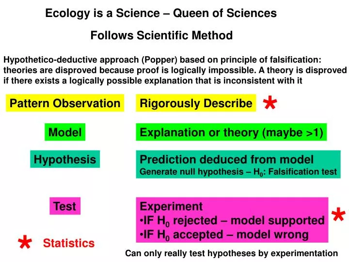
1. * Pattern Observation Rigorously Describe Model Explanation or theory (maybe >1) Hypothesis Prediction deduced from model Generate null hypothesis – H0: Falsification test * Test • Experiment • IF H0 rejected – model supported • IF H0 accepted – model wrong * Statistics Ecology is a Science – Queen of Sciences Follows Scientific Method Hypothetico-deductive approach (Popper) based on principle of falsification: theories are disproved because proof is logically impossible. A theory is disproved if there exists a logically possible explanation that is inconsistent with it Can only really test hypotheses by experimentation

2. Give off light when attacked by copepods to attract fish (to eat the copepods) Model Explanation or theory (maybe >1) Hypothesis Prediction deduced from model Generate null hypothesis – H0: Falsification test H0: Bioluminescence has no effect on predation of copepods by fish (or decreases predation) H1: Bioluminescence increases predation of copepods by fish • Experiment • IF H0 rejected – model supported • IF H0 accepted – model wrong Test Notiluca give off light when disturbed Pattern Observation Rigorously Describe

3. Statistics – summary, analysis and interpretation of data Data pl (datum, s) are observations, numerical facts RAW MATERIAL OF SCIENCE Types of Data Nominal data – gender, colour, species, genus, class, town, country, model etc Continuous data – concentration, depth, height, weight, temperature, rate etc Discrete data – numbers per unit space, numbers per entity etc Often referred to as VARIABLES because they vary The type of data collected influences their analysis

4. Variability – key feature of the natural world Genotypic/Phenotypic variation – differences between individuals of the same species (blood-type, colour, height etc) Variability in time/space – changes in numbers per unit space, time Uniform Random Clumped Space/Time Measurement variability – experimental error (bias)

5. Variability = Uncertainty Variability means that it is impossible to describe data exactly –Accuracy, Precision

6. 20 cm + 6 mm + 300 μm + Accuracy – how close a measure is to the real value 20.63 cm 20.631506542 cm Accept a level of measurement error: be upfront

7. 20.755 20.632 20.623 21.102 20.710 19.986 22.356 20.493 20.578 Precision – how close repeat measures are to each other

8. Describing data and variability Population – the entire collection of measurements, e.g. mass of 19 yr old elephants, the blood pressure of women between 16-18 yrs of age, number of earthworms on UWC rugby field, height of UWC BSc II students, oxygen content of water If population small, then possible to obtain all measurements in the population. However, if population very large, then impractical or impossible to measure all - must take Samples One sample from a large population is meaningless –need to take replicate samples and obtain an average sample measure, which is then assumed to be representative of the population When taking samples it is vital that they are Random and Independent

9. Earthworms D C B A 100 m 100 m How many earthworms in the field of 25 0000 m2? 500 m A – 1 (25) B – 17 (375) C – 10 (250) D – 4 (100) Mean = 8 (200) 500 m

10. N = 106 Σ = 182.4 Mean = 1.72 Mean = Σx N Population mean = μ; sample mean = x We use x as a proxy for μ Describing data and variability How high is a UWC BSc II student? What is the NO3 concentration in the Black River? Measures of Central Tendency Arithmetic mean or Average

11. =COUNT(DATA:RANGE) =SUM(DATA:RANGE) =TOTAL / N MSExcel also allows you to calculate the mean from a data series… =AVERAGE(DATA:RANGE) Enter data (x) into MSExcel spreadsheet Calculate N Calculate Total Calculate Mean

12. Mode – the most commonly represented value How? Construct a frequency table from the data: whichever “class” of data occurs at the highest frequency is the MODE Classes should be calculated in EVEN intervals from smallest to largest value of x MSExcel allows you to calculate a frequency table It also allows you to calculate MODE: = MODE(DATA:RANGE)

13. UNIMODAL BIMODAL TRIMODAL

14. If there are an odd number of data points this is easy If there are an even number of data points you will need to interpolate The middle data point lies half way between that associated with observation no 5 (1.75) and observation no 6 (1.8) = 1.775 Can be calculated as either (1.75 + 1.8) / 2 OR as ((1.8 – 1.75) / 2) + 1.75 MSExcel also allows you to calculate the median from a data series… =MEDIAN(DATA:RANGE) Median – the middle value in a ranked data set Step 1 – Order the data from low to high Step 2 – Determine the middle data point

15. Range: Essentially the lowest and highest value in the data set Measures of Dispersion – how data are distributed around the mean N.B. Subject to measurement errors, typographic mistakes and freaks In MSExcel: =MIN(DATA:RANGE), =MAX(DATA:RANGE)

16. ¼ of the way through this ranked data set of 9 values = observation number 2.25 (=9 x 0.25) Calculate the data point that would be associated with observation number 2.25 by interpolation between observation numbers 2 (1.45) and 3 (1.6) i.e. = ((1.6 – 1.45) * 0.25) + 1.45 = ((0.15) * 0.25) + 1.45 = 0.0375 + 1.45 = 1.4875 (Lower Quartile) Inter-Quartile Range: In a ranked data set, those values corresponding to ¼ (lower or 25% quartile) and ¾ (upper or 75% quartile) of the observations: 50% of the observations lie between these two values DITTO for 75% Quartile……………….. To give us an interquartile range: 1.4875 – 1.8875 If you have to use a range, use the inter-quartile range as it ignores outliers

17. MEDIAN LOWER UPPER Can also calculate Cumulative Frequency THEN Draw a Graph of Cumulative Frequency (Y) against Ordered Data (X) on an X-Y PLOT THEN Calculate Lower and Upper Quartiles from Figure

18. Always = Zero Mean Deviation Σ Convert negatives to positives to give overall deviation from the mean; SUM, Divide by N to give average deviation of any data point from the mean – MEAN DEVIATION N mean

19. Always = Zero The values of x = 4, sample variance (2.25) and sample standard deviation (1.5) ALL refer to the sample of 16 measures Sum of Squares (Sample) Mean Sum of Squares (sample) (Variance) Σ Σ Σ √ N N N (Variance) = mean mean mean Standard Deviation (sample) s = 1.5 16 2.25 Length (mm) of Drosophila melanogaster Instar III larvae Variance and Standard Deviation There is another way to remove the negatives – and that is to square the (x – mean) values Square units?

20. X 3 If you had collected only the first four of the measures (in pink), then the total would be 18. In order for you to get a mean of 5 from five measures, the last value would HAVE TO BE seven (7). In other words the last number is not independent of the others, and when we deal with the population we have to use independent data. Consequently when we calculate σ2 we divide the sum of squares by (n-1) and NOT n (as previously): σ is still calculated as In this table of five measures, the total is 25 and x is 5 4 X 5 3 6 4 7 5 6 Total 25 7 N 5 Mean 5 Total 25 N 5 Mean 5 √ σ2 Are they the best estimators of these properties for the population? In the case of the mean (x), there is no reason to suppose that the mean of all observations in the sample will not provide the best estimator of the population mean (μ) However, we cannot use sample variance and sample standard deviation as estimators of σ2 and σ respectively! WHY? Because not all the measures are completely independent of each other. (n-1) = Degrees of Freedom = v Sample derived estimates of population variance and population standard deviation are referred to as s2 and s respectively

21. Mean N s2 s The smaller the standard deviation, the closer the data are to the mean The bigger the standard deviation, the greater the spread of data around the mean – the greater the variability

22. So…… Mean – measure of central tendency of sample data Variance and Standard Deviation – index of dispersion of data around the sample and/or population mean Two other commonly reported measures of central tendency: Standard Error – index of dispersion of sample means around population mean 95% confidence intervals – describes limits around your sample mean within which you are 95% confident that the REAL value of the population mean lies To calculate the last two measures, it is necessary to digress a little……

23. A die has six sides: The probability of throwing = 1/6 = 0.167 The probability of NOT throwing a = 1 – 0.167 = 0.833 Variability = Uncertainty View uncertainty in terms of probability • What is the probability of a particular event occurring? • What is the probability of a particular observation being made? NB – the sum of probabilities = 1.0 A coin has two sides: 1 heads and 1 tails: 1 + 1 = 2 The probability of throwing heads = ½ = 0.5 P(heads) = 0.5 P(tails) = 1 – P(heads) = 1 – 0.5 = 0.5

24. 16 14 12 10 8 Frequency 6 4 2 0 2 1.2 1.3 1.4 1.5 1.6 1.7 1.8 1.9 2.1 2.2 Height (m) What is probability the picking a student of 1.65 m high from the class? Depends on how the data are distributed If the total number of students in the class is 106, and 10 of them are 1.65 m high, then the chance of picking (at random) a student measuring 1.65 m is 10 in 106: P(1.65) = 0.094 If the total number of students in the class is 106, and 96 (106-10) of them are NOT 1.65 m high, then the chance of picking (at random) a student NOT measuring 1.65 m is 96 in 106: P(NOT 1.65) = 0.906 P(NOT 1.65) = 1 – P(1.65) = 1 – 0.094 = 0.906

25. When data are displayed as a frequency distribution, the area under any part of the curve reflects the number of observations involved. In this case, 10 observations are of 1.65 m (in red) 96 (in blue) are not 16 14 12 10 16 8 Frequency (%) 14 6 12 4 10 2 8 Frequency 0 6 2 1.2 1.3 1.4 1.5 1.6 1.7 1.8 1.9 2.1 2.2 4 Frequency distributions do not only have to be displayed in terms of numbers, they can also be displayed as proportions or percentages. Height (m) 2 0 2 1.2 1.3 1.4 1.5 1.6 1.7 1.8 1.9 2.1 2.2 Height (m) Same rules – the area under any part of the curve reflects the proportion of observations involved...or PROBABILITIES In this case, 0.094 (9.4%) are of 1.65 m (in red) and 0.906 (90.6%) are not (in blue) The total area under the curve = the total number of observations The total area under the curve = 1.0

26. 16 14 12 10 8 Frequency (%) 6 4 2 0 2 1.2 1.3 1.4 1.5 1.6 1.7 1.8 1.9 2.1 2.2 Height (m) Most of the data are clustered around the mean, which means that there is a fairly good chance (high probability) of your picking at random from the class a student with a height close to the mean On the other hand, there is a relatively small chance that you will pick a student (by random) that is either very tall or very short: i.e. those whose measures are located in the tails of the distribution

27. 500 12 N = 4064 10 Σ = 100% 400 8 300 6 Frequency (%) Frequency 200 4 2 100 0 0 0 2 4 6 8 10 12 14 16 18 20 22 24 0 2 4 6 8 10 12 14 16 18 20 22 24 No Worms per quadrat No Worms per quadrat The shape of the curve depends on the variance or standard deviation: the spread of values about the mean Mean = 10 Most data that scientists collect is what we call normally distributed – but NOT all. s2 = 4 s2 = 8 s2 = 12 s2 = 16

28. 12 10 Σ = 100% 8 6 Frequency (%) 4 2 0 0 2 4 6 8 10 12 14 16 18 20 22 24 No Worms per quadrat • For data that are normally distributed: • The mean, median and mode are the same • The frequency distribution is completely symmetrical either side of the mean • The area under the curve is proportional to number of observations • The normal curve has fixed mathematical properties, irrespective of • The scale on which it is drawn • The magnitude or units of its mean • The magnitude or units of its Standard Deviation • …….and these render it susceptible to statistical analysis

29. Z = (x – μ) σ Calculating proportions of a Normal Distribution To calculate the probability of a particular value x being drawn from a normally distributed population of data, you need to know the mean AND the standard deviation of the data Equation 1 μ = population mean, σ = population standard deviation What Z describes is the difference between the mean and any value x, expressed as a proportion of the standard deviation, i.e. how many standard deviations away from the mean is the value x Obviously, the smaller the value of Z, the closer the value of x is to the mean Because Z is based on data that are normally distributed, it too is normally distributed (the Z distribution). With a knowledge of Z, we can go to statistical tables drawn up based on the normal distribution and calculate the associated probability

30. Frequency Z = 1.33 Z = (x – μ) 0.45 0.55 0.65 0.75 0.85 0.95 1.05 1.15 1.25 1.35 1.45 1.55 1.65 1.75 1.85 1.95 2.05 2.15 2.25 2.35 2.45 2.55 Height (m) σ Z = (0.4) Z = (1.95 – 1.55) 0.3 0.3 Frequency 0.00 0.33 0.67 1.00 1.33 1.67 2.00 2.33 2.67 3.00 3.33 -3.67 -3.33 -3.00 -2.67 -2.33 -2.00 -1.67 -1.33 -1.00 -0.67 -0.33 Z e.g. if μ = 1.55 m, σ = 0.3 m, what is the probability of a student measuring more than 1.95 m being drawn at random from the population? ? A student measuring 1.95 m is 1.33 times the standard deviation away from the mean, and this corresponds to a value of 0.0918 from the Z Tables 0.0918

31. n N 16 15 14 13 12 11 10 9 8 7 6 5 4 σ2 σ2 σ2 = = population variance of the mean x x n The Distribution of Means If random samples of size n are drawn from a normal population, the means of those samples will form a normal distribution The variance of the distribution of means will decrease as n increases Equation 2

32. Just as is a normal deviate referring to the normal distribution of Xi values σ = √ Z = (x – μ) n σ So is a normal deviate referring to the normal distribution of means σ2 √ = Z = (x – μ) n 4 4 N = 9, X = 50.0 mm, μ = 47.0 mm, σ = 12.0 mm Z = (50.0 – 47.0) = 3 = 0.75 = 4 √ = 12.0 = 12 9 σ σ σ σ 3 = standard error of the mean x x x x So… What is the probability of obtaining a random sample of nine measurements with a mean greater than 50.0 mm, from a population having a mean of 47 mm and a standard deviation of 12.0 mm?

33. What is the probability of obtaining a random sample of nine measurements with a mean greater than 50.0 mm, from a population having a mean of 47 mm and a standard deviation of 12.0 mm? 4 4 N = 9, X = 50.0 mm, μ = 47.0 mm, σ = 12.0 mm Z = (50.0 – 47.0) = 3 = 0.75 = 4 √ = 12.0 = 12 9 σ 3 x Looking up 0.75 on the Z Tables gives – 0.2266

34. The observant amongst you will have noted that in the last couple of equations for Z we have used the population parameters: μ, σ and Trouble is we don’t usually have access to population data and must make do with sample estimators x, s and IF n is large: we use Z distribution to calculate normal deviates = Z = (x – μ) t = (x – μ) V = 100 V = 10 V = 5 V = 1 s s σ s σ σ -9 -8 -7 -6 -5 -4 -3 -2 -1 0 1 2 3 4 5 6 7 8 9 x x x x x x t Equation 3 IF n is small, then must use t distribution: Shape of the t distribution varies with v (Degrees of Freedom: n-1): the bigger the n, the less spread the distribution t distribution given rise to many statistical tests!

35. α (1) α (1) 0.1 0.1 -4 -3 - 2 -1 0 1 2 3 4 -4 -3 - 2 -1 0 1 2 3 4 t 1.372 -1.372 t α (2) 0.05 0.05 - 2 -4 -3 -1 0 1 2 3 4 t -1.812 1.812 One-Tailed Two-Tailed • Because it is based on the normal distribution, the t distribution has all the attributes of the normal distribution: • Completely symmetrical • Area under any part of the curve reflects proportion of t values involved • etc…. For a particular area of the curve we can calculate the associated t values, using t-tables at the end of most text books on statistics For example: if our sample size is 11 (v = 10), what is the value of t beyond which 10% (0.1) of the curve is enclosed? – Two possible answers

36. α (1) α (2) 0.1 0.05 0.05 - 2 -4 -3 -1 0 1 2 3 4 -4 -3 - 2 -1 0 1 2 3 4 t -1.372 t -1.812 1.812 One-Tailed Two-Tailed How do you get the t values from the t-tables?

37. s = √ n H0: μ = 22 H1: μ ≠ 22 t = (x – μ) How? – use t-test = = = 2.629 2.23 (24.23 – 22) 0.848 0.848 x = 24.23 s = 4.24 μ = 22.00 n = 25 4.24 4.24 = = √ 5 25 = 0.848 s s x x The mean nitrate concentration of water in all the upstream tributaries of a large river prior to intensive agriculture is 22 mg.l-1. Afterwards the mean nitrate concentration in 25 of these tributaries is 24.23 mg.l-1 and s = 4.24 mg.l-1 We can now use the t distribution to demonstrate the term statistical significance – which is something that you will get confronted with regularly when reading EIA reports… This is an observation, and we want to determine if the intensification of agricultural practices has resulted in any change to the nitrate concentration of the freshwater resources. Step 1: establish the hypotheses Step 2: Need to determine the probability that a random sample (size 25) will generate a mean of 24.23 mg.l-1 from a population with a mean of 22 mg.l-1?

38. α (1) α (2) H0: μ = 22 H1: μ ≠ 22 0.05 0.025 0.025 t t One-Tailed Two-Tailed Go to the hypotheses Step 3: Determine, from the t-tables, the (critical) value of t, beyond which we consider such a random sample mean as being unlikely Generally we consider an event as being unlikely if it occurs in the extreme 5% of the normal distribution So we need to determine the (critical) value of t, beyond which 5% of the curve is enclosed – for v = 24 But do we use α (1) or α (2)?

39. The critical value of t, α (2) 0.05, v = 24, is 2.064 0.025 0.025 -4 -3 - 2 -1 0 1 2 3 4 t -2.064 2.064 2.629 Our value of t is 2.629, which lies beyond the critical value of t That means it is very unlikely that a random sample (size 25) would generate a mean of 24.23 mg.l-1 from a population with a mean of 22 mg.l-1 So unlikely, in fact, that we don’t believe it can happen by chance Reject H0 and accept H1

40. What we can then say, is that the before and after nitrate levels in the water are (statistically) significantly different from each other (p < 0.05) We are not making any judgment about whether there is more nitrate in the water after than before, only that the concentrations are different – though some things are self evident! You will frequently come across the terms p<0.05, p<0.01: these mean that the probability of a particular event occurring by chance alone are less than 5% and 1% respectively, which is unlikely On the other hand if results are reported as p>0.05, it means that the probability of a particular event occurring by chance alone is greater than 5%, which is possible.

41. The t-Distribution allows us to calculate the 95% (or 99%) confidence intervals around an estimate of the population mean In other words, what are limits around our estimate of the population mean, WITHIN which we 95% (or 99%) confident that the REAL value of the population mean lies α (2) 0.025 0.025 t Two-Tailed To do this, we need a set of t-tables, and V (N-1) s s x x t = (x – μ) * Difference between population and sample mean

42. IF = 42.3 mm N = 26 (V = 25) = 2.15 * t = 2.15 *2.06 = 4.429 ά 2 The expression is then written as: 42.3 mm 4.43 mm ± To do this, we need a set of t-tables, and V (N-1) s s s x x x x Then the 95% CI around the mean will be

43. 16 14 12 You can covert continuous data to discrete data, by assigning data to data classes 10 8 Frequency 6 4 2 0 2 1.2 1.3 1.4 1.5 1.6 1.7 1.8 1.9 2.1 2.2 Height (m) Testing Patterns in Discrete (count) Data: the Chi-Square Test Examples of count data: Number of petals per flower Number of segments per insect leg Number of worms per quadrat Number of white cars on campus etc

44. Often want to determine if the population from which you have obtained count data conform to a certain prediction DATA DO NOT HAVE TO BE NORMALLY DISTRIBUTED For Example: A geneticist has raised 134 progeny from a cross that is hypothesized to result in a 3:1 ratio of yellow-flowered to green-flowered plants. She counts 113 yellow-flowering and 21 green-flowering plants amongst the progeny Theoretically she should have obtained 100.5 yellow-flowering plants and 33.5 green-flowering plants (100.5 = 134 x 0.75, 33.5 = 134 x 0.25: 0.75 =3/ (3+1), 0.25 =1/ (3+1)) Does the OBSERVED ratio (113:21) differ (SIGNIFICANTLY) from the Expected (100.5:33.5) ratio? Establish Hypotheses H0: Population sampled has yellow:green flowering plants in ratio 3:1 H1: Population sampled does not have yellow:green flowering plants in ratio 3:1

45. χ χ χ 2 2 2 Does the OBSERVED ratio (113:21) differ (SIGNIFICANTLY) from the Expected (100.5:33.5) ratio? [ ] [ ] (113 – 100.5)2 (21 – 33.5)2 = 1.55 + 4.66 = 6.22 + = 100.5 33.5 [ ] 2 Σ (O – E) = Equation 4 E Where O = Observed, E = Expected Obviously, the bigger the difference between O and E, the greater the When there is no difference, the value will be ZERO: hence Goodness of Fit NB: MUST ALWAYS USE FREQUENCIES: not PERCENTAGES OR PROPORTIONS

46. χ χ χ 2 2 2 Our value of greater than that corresponding to 0.025 (2.5%) but less than that corresponding to 0.01 (1%) – from the Tables. Do we accept or reject the Null Hypothesis? [ ] [ ] (113 – 100.5)2 (21 – 33.5)2 = 1.55 + 4.66 = 6.22 + = 100.5 33.5 Degrees of Freedom (v) = K – 1, where K = Number of categories (in this case two: yellow-flowering or green-flowering) = 2 – 1 = 1

47. A plant geneticist has done some crossing between plants and come up with the following numbers of different seeds Has the geneticist sampled from a population having a ratio of 9:3:3:1 ? What are the hypotheses being tested? How many degrees of freedom are there? H0: Population sampled has YS:YW:GS:GW seeds in the ratio 9:3:3:1 H1: Population sampled does not have YS:YW:GS:GW seeds in the ratio 9:3:3:1 K – 1 = 4 – 1 = 3

48. χ χ χ 2 2 2 = 8.97 What is the critical value of Our value of is greater than the critical value: Reject the Null Hypothesis that sample drawn from a population showing 9:3:3:1 ratio of YS:YW:GS:GW

49. χ 2 The greatest contributor to the value is GW v = K – 1 = 3 – 1 = 2 You can go further – and look to find whereabouts the pattern fails to conform to predictions Do the other observations conform to the ratio 9:3:3 (YS:YW:GS)? Establish Hypotheses YES

50. v = K - 1 = 2 – 1 = 1 Having confirmed that the observations fit the model (9:3:3), we can now combine them and test if the ratio of GW to the others is 1:15 Establish Hypotheses Reject Null Hypothesis and draw the conclusion that there is a problem with GW