Download
1 / 17
410 likes | 1.08k Views
Image processing. Scene analysis. Bitmap image. feedback (tuning). Prepare image for scene analysis. Build an iconic model of the world. Computer Vision. A simple two-stage model of computer vision:. Scene description. Computer Vision.

E N D
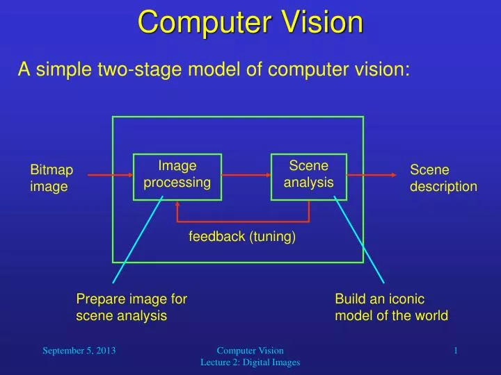
Image processing Sceneanalysis Bitmap image feedback (tuning) Prepare image for scene analysis Build an iconic model of the world Computer Vision • A simple two-stage model of computer vision: Scene description Computer Vision Lecture 2: Digital Images
Computer Vision • The image processing stage prepares the input image for the subsequent scene analysis. • Usually, image processing results in one or more new images that contain specific information on relevant features of the input image. • The information in the output images is arranged in the same way as in the input image. For example, in the upper left corner in the output images we find information about the upper left corner in the input image. Computer Vision Lecture 2: Digital Images
Computer Vision • The scene analysis stage interprets the results from the image processing stage. • Its output completely depends on the problem that the computer vision system is supposed to solve. • For example, it could be the number of bacteria in a microscopic image, or the identity of a person whose retinal scan was input to the system. • In the following lectures we will focus on the lower-level, i.e., image processing techniques. • Later we will discuss a variety of scene analysis methods and algorithms. Computer Vision Lecture 2: Digital Images
Computer Vision • How can we turn a visual scene into something that can be algorithmically processed? • Usually, we map the visual scene onto a two-dimensional array of intensities. • In the first step, we have to project the scene onto a plane. • This projection can be most easily understood by imagining a transparent plane between the observer (camera) and the visual scene. • The intensities from the scene are projected onto the plane by moving them along a straight line from their initial position to the observer. • The result will be a two-dimensional projection of the three-dimensional scene as it is seen by the observer. Computer Vision Lecture 2: Digital Images
(x, y, z) y’ y (x’, y’) z f x x’ Digitizing Visual Scenes • Obviously, any 3D point (x, y, z) is mapped onto a 2D point (x’, y’) by the following equations: Computer Vision Lecture 2: Digital Images
Digitizing Visual Scenes • Once we obtained the 2D projection of our scene, it is still not ready for storage in our computer. • The image theoretically has infinite spatial resolution and an infinite number of colors. • We will mostly restrict our concept of images to grayscale. • Grayscale values usually have a resolution of 8 bits (256 different values), in medical applications sometimes 12 bits (4096 values), or in binary images only 1 bit (2 values). • We simply choose the available gray level whose intensity is closest to the gray value color we want to convert. Computer Vision Lecture 2: Digital Images
y’ [0, 0] [0, 1] [0, 2] [0, 3] [1, 0] [1, 1] [1, 2] [1, 3] [2, 0] [2, 1] [2, 2] [2, 3] x’ Digitizing Visual Scenes • With regard to spatial resolution, we will map the intensity in our image onto a two-dimensional finite array: Computer Vision Lecture 2: Digital Images
Digitizing Visual Scenes • So the result of our digitization is a two-dimensional array of discrete intensity values. • Notice that in such a digitized image F[i, j] • the first coordinate i indicates the row of a pixel, starting with 0, • the second coordinate j indicates the column of a pixel, starting with 0. • In an m×n pixel array, the relationship between image and pixel coordinates is given by the equations Computer Vision Lecture 2: Digital Images
Levels of Computation • As we discussed before, computer vision systems usually operate at various levels of computation. • In the following, we will discuss different levels of computation as they occur during the image processing and scene analysis stages. • We will formalize this concept by means of an operation O that receives a set of pixels and returns a single intensity value that can be used to determine the value of a pixel in the output image. • We will look at operations at the point level, local level, global level, and object level mapping an input image fA[i, j] to an output image fB [i, j]. Computer Vision Lecture 2: Digital Images
Point Level • Operation type: • fB[i, j] = Opoint{fA[i, j]} • This means that the intensity of each pixel in the output image only depends on the intensity of the corresponding pixel in the input image. • Examples for this kind of operation are inversion (creating a negative image), thresholding, darkening, increasing brightness etc. Computer Vision Lecture 2: Digital Images
Local Level • Operation type: • fB[i, j] = Olocal{fA[k, l]; [k, l] N[i, j]} • Where N[i, j] is a neighborhood around the position [i, j]. For example, it could be defined as • N[i, j] = {[u, v] | |i – u| < 3 |j – v| < 3}. • Then the neighborhood would include all pixels within a 5×5 square centered at [i, j]. • So the intensity of each pixel in the output image depends on the intensity of pixels in the neighborhood of the corresponding position in the input image: • Examples: Blurring, sharpening. Computer Vision Lecture 2: Digital Images
Global Level • Operation type: • fB[i, j] = Oglobal{fA[k, l]; 0 ≤ k < m, 0 ≤ l < n} • for an m×n image. • So the intensity of each pixel in the output image may depend on the intensity of any pixel in the input image. • Examples: histogram modification, rotating the image Computer Vision Lecture 2: Digital Images
Object Level • The goal of computer vision algorithms usually is to determine properties of an image with regard to specific objects shown in it. • To do this, operations must be performed at the object level, that is, include all pixels that belong to a particular object. • Problem: We must use all points that belong to an object to determine its properties, but we need some of these properties to determine the pixels that belong to the object. • While this seems effortless in biological systems, we will later see that complex algorithms are required to solve this problem in an artificial system. Computer Vision Lecture 2: Digital Images
Binary Images • Binary images are grayscale images with only two possible levels of brightness for each pixel: black or white. • Binary images require little memory for storage and can be processed very quickly. • They are a good representation of an object if • we are only interested in the contour of that object, and • the object can be separated from the background and from other objects (no occlusion). Computer Vision Lecture 2: Digital Images
Thresholding • We usually create binary images from grayscale images through thresholding. • This can be done easily and perfectly if, for example, the brightness of pixels is lower for those of the object than for those of the background. • Then we can set a threshold T such that T is • greater than the brightness value of any object pixel and • smaller than the brightness value of any background pixel. Computer Vision Lecture 2: Digital Images
Thresholding • In that case, we can apply the threshold T to the original image F[i, j] to generate the thresholded image FT[i, j]: • FT[i, j] = 1 if F[i, j] ≤ T = 0 otherwise • The convention for binary images is that pixels belonging to the object(s) have value 1 and all other pixels have value 0. • We usually display 1-pixels in black and 0-pixels in white. Computer Vision Lecture 2: Digital Images
Thresholding • If we know that the intensity of all object pixels is in the range between values T1 and T2, we can perform the following thresholding operation: • FT[i, j] = 1 if T1≤ F[i, j] ≤ T2 = 0 otherwise • If the intensities of all object pixels are not in a particular interval, but are still distinct from the background values, we can do the following: • FT[i, j] = 1 if F[i, j] Z = 0 otherwise, • Where Z is the set of intensities of object pixels. Computer Vision Lecture 2: Digital Images