Download
1 / 194
1.95k likes | 2.11k Views
The World Distribution of Income (from Log-Normal Country Distributions). Xavier Sala-i-Martin Columbia University April 2010. Goal. Estimate WDI consistent with the empirical growth evidence (which uses GDP per capita as the mean of each country/year distribution).

E N D
The World Distribution of Income (from Log-Normal Country Distributions) Xavier Sala-i-Martin Columbia University April 2010
Goal • Estimate WDI consistent with the empirical growth evidence (which uses GDP per capita as the mean of each country/year distribution). • Estimate Poverty Rates and Counts resulting from this distribution • Estimate Income Inequality across the world’s citizens • Estimate welfare across the world’s citizens • Analyze the relation between poverty and growth, poverty and inequality
Data • GDP Per capita (PPP-Adjusted –See Note next page). • We usually use these data as the “mean” of each country/year distribution of income (for example, when we estimate growth regressions)
Note: I decompose China and India into Rural and Urban • Use local surveys to get relative incomes of rural and urban • Apply the ratio to PWT GDP and estimate per capita income in Rural and Urban and treat them as separate data points (as if they were different “countries”) • Using GDP Per Capita we know…
But NA Numbers do not show Personal Situation: Need Individual Income Distribution • We can use Survey Data • Problem • Not available for every year • Not available for every country • Survey means do not coincide with NA means
Surveys not available every year • Can Interpolate Income Shares (they are slow moving animals) • Regression • Near-Observation • Cubic Interpolation • Others
Missing Countries • Can approximate using neighboring countries
Method: Interpolate Income Shares • Break up our sample of countries into regions(World Bank region definitions). • Interpolate the quintile shares for country-years with no data, according to the following scheme, and in the following order: • Group I – countries with several years of distribution data • We calculate quintile shares of years with no income distribution data that are WITHIN the range of the set of years with data by cubic spline interpolation of the quintile share time series for the country. • We calculate quintile shares of years with no data that are OUTSIDE this range by assuming that the share of each quintile rises each year after the data time series ends by beta/2^i, where i is the number of years after the series ends, and beta is the coefficient of the slope of the OLS regression of the data time series on a constant and on the year variable. This extrapolation adjustment ensures that 1) the trend in the evolution of each quintile share is maintained for the first few years after data ends, and 2) the shares eventually attain their all-time average values, which is the best extrapolation that we could make of them for years far outside the range of our sample. • Group II – countries with only one year of distribution data. • We keep the single year of data, and impute the quintile shares for other years to have the same deviations from this year as does the average quintile share time series taken over all Group I countries in the given region, relative to the year for which we have data for the given country. Thus, we assume that the country’s inequality dynamics are the same as those of its region, but we use the single data point to determine the level of the country’s income distribution. • Group III – countries with no distribution data. • We impute the average quintile share time series taken over all Group I countries in the given region.
Method 2: Step 1: Find the σof the lognormal distribution using least squares for the country/years with survey data
Step 2: Compute the resulting normal distributions for each country-year
Step 3: Estimate implied Gini coefficients for country/years with available surveys
Step 4: Three Types of countries • Countries with multiple surveys • Intrapolateginis • Estimate location parameter as a function of sigma(Gini) for intrapolated years and then estimate the mean with sigma and GDP per capita • Countries with ONE survey • We keep the single year of data, and impute the Ginis for other years to have the same deviations from this year as does the average Gini time series taken over all Group I countries in the given region, relative to the year for which we have data for the given country (ie, we assume that the country’s inequality dynamics are the same as those of its region, but we use the single data point to determine the level of the country’s income distribution.) • Countries with NO distribution data • We impute the average Gini time series taken over all Group I countries in the given region.
Summary of Baseline Assumptions • We use GDP data from PWT 6.2 • Sensitivity: WB, Madison • We break up China and India into urban and rural components, and use POVCAL surveys for within country inequality. • Sensitivity: China and India are treated as unitary countries • We use piecewise cubic splines to interpolate between available survey data, and extrapolate by horizontal projection. • Sensitivity Interpolation: 1) nearest-neighbor interpolation, 2) linear interpolation. • Sensitivity Extrapolation: 1) assuming that the trends closest to the extrapolation period in the survey data continue unabated and extrapolating linearly using the slope of the Gini coefficient between the last two data points, and 2) a mixture of the two methods in which we assume the Gini coefficient to remain constant into the extrapolation period, except if the last two years before the extrapolation period both have true survey data. • Lognormal distributions • Sensitivity: 1) Gamma, 2) Weibull, 3) Optimal (Minimum Squares of residuals), 4) Kernels