Download

1 / 43
430 likes | 886 Views
Course : COMP7116 - Computer Vision Effective Period : February 2018. Image Feature Session 0 7. Learning Objectives. After carefully listening this lecture, students will be able to do the following :

E N D
Course : COMP7116 - Computer Vision Effective Period : February 2018 Image FeatureSession 07
Learning Objectives • After carefully listening this lecture, students will be able to do the following : • Describe the computational principles underlying various application of Computer Vision Systems • Select and extract different image features required for various application of Computer Vision Systems
Outline Interest Points Local Features components Harris Corner Detection
Interest Points ORB (Oriented FAST and Rotated BRIEF) • Note: “interest points” = “keypoints”, also sometimes called “features” • Many applications • tracking: which points are good to track? • recognition: find patches likely to tell us something about object category • 3D reconstruction: find correspondences across different views
ORB (Oriented FAST and Rotated BRIEF) ORB is basically a fusion of FAST keypoint detector and BRIEF descriptor with many modifications to enhance the performance. First it use FAST to find keypoints, then apply Harris corner measure to find top N points among them. It also use pyramid to produce multiscale-features. But one problem is that, FAST doesn’t compute the orientation. So what about rotation invariance? Authors came up with following modification.
Feature Detection https://pysource.com/2018/03/21/feature-detection-sift-surf-obr-opencv-3-4-with-python-3-tutorial-25/
Overview of Keypoint Matching Find a set of distinctive key-points 2. Define a regionaround each keypoint A1 B3 3. Extract and normalize the region content A2 A3 B2 B1 4. Compute a local descriptor from the normalized region 5. Match local descriptors
Goals of Keypoints Detects points that are repeatable and distinctive.
Key Trade-offs Detection of interest points Description of patches
Invariant Local Features Image content is transformed into local feature coordinates that are invariant to translation, rotation, scale and other imaging parameters. Features Descriptors
Local Features : Main Components • Detection: Identify the interest points • Description: Extract vector feature descriptor surrounding each interest point. • Matching: Determine correspondence between descriptors in two views
Characteristics of Good Features • Repeatability • The same feature can be found in several images despite geometric and photometric transformations • Saliency • Each feature is distinctive • Compactness and efficiency • Many fewer features than image pixels • Locality • A feature occupies a relatively small area of the image; robust to clutter and occlusion
“flat” region:no change in all directions “edge”:no change along the edge direction Corner Detection : Basic Idea • We should easily recognize the point by looking through a small window • Shifting a window in anydirection should give a large change in intensity “corner”:significant change in all directions
Corner Detection : Basic Idea • Key property: in the region around a corner, image gradient has two or more dominant directions • Corners are repeatable and distinctive C.Harris and M.Stephens. "A Combined Corner and Edge Detector.“Proceedings of the 4th Alvey Vision Conference: pages 147--151.
Harris Corner Detector Procedures 12pixels Pixel(x,y) 12 pixels N= Neighborhood (12x12) window • Harris Algorithm • Scan through all x,y in the image • For each pixel (x,y) find the neighborhood N(x,y) which is a (12x12) window. • Inside N(x,y) a 12x12 window, Find A • Find Eigen 2 values of A(x,y)=max, min • Sort all min , discard pixel with small min. • Discard pixels with large max- min.. • Remaining are corner points
Interpreting the Eigenvalues Vertical Edges (max >> min) Corner area (max min) And they are large enough min max, min are small Horizontal Edges (max >> min) “Flat” region max
Ex : Tracking/Matching by Correlation Image1 (at Time=1)Image2 (at time=2) gi(j=2) fi:a small window gi(j=1) ri,j=1= correlation(fi,gi(j=1)) ri,j=2= correlation(fi,gi(j=2))
Ex : A Stereo System Left image Right image A corner feature is foundin a 10x10 window (w) centered at the left image (xL,yL) (overlay a cross) Horizontal search range=dx (around [xL,yL]) For (x’=xR-dx; x’<xR;x’=x’+1) { w’=a 10x10 window centered at (x’,yL) c(x’)=Correlate (w,w’) } Find index of max {for all c(x’)}= xR”. then the corresponding window is centered at (xR”,yL) Horizontal disparity = (xL-xR”)
Connected Components X’ Y’ Y X X and Y are connected X’ and Y’ are NOT connected a and b are connected if there exists a path from a to b Notation: if a and b are connected, we write a ~ b
Connected Components • Two pixels are c-adjacent (c=4 or 8) if they share at least an edge (c=4), or a vertex (c=8). • Two pixels are c-connected (c=4 or 8) if it is possible to find a path between these two pixels through pairs of c-adjacent (c=4,8) pixels. • A c-connected component is a maximal connected set where each pixel is c-connected to other pixels in the set.
Ex of Connected Components q q p p p ~ q no matter 4-neighbors or 8-neighbors p ~ q only when 8-neighbors is considered
Component Labeling original binary image If 4-neighbors, 3 connected components If 8-neighbors, 2 connected components
CC Algorithm • Process the image row by row • Assign a label to the first pixel of each CC • Otherwise assign its label by propagating from left or top 1 2 1 2 1 1 2 1 1 1 ? Clash!
One approach • Propagate the smaller label in case of clash • Record the equivalence in a table • After the entire image is processed, find the set of equivalence classes • Second pass replaces each label with its equivalent class TWO PASSES!
Ex : Object Extraction • Since the input is a color image, we first covert it to • gray level image before moving to further processing.
Ex : Object Extraction • In order to improve segmentation accuracies, we have to eliminate noise. To do this, we are applying the well known median filtering. After removing the noise, we then employ Sobel edge detector to reveal the edges of the input image
Ex : Object Extraction • We still need to eliminate the unnecessary connected components by smoothing the image using box filter. • Next, we apply 8-neighborhood approach to get the number of connected components.
_ + Boundary of Binary Objects X X X=X-(X B) X=(X B) – B or
Chain Codes Boundary Representation 4-directional chain code: 0033333323221211101101 8-directional chain code: 076666553321212
Two Problems with the Chain Code • Chain code representation is conceptually appealing, yet has the following two problems • Dependent on the starting point • Dependent on the orientation • To use boundary representation in object recognition, we need to achieve invariance to starting point and orientation • Normalized codes • Differential codes
Normalization Strategy 33001122 33001122 30011223 00112233 01122330 11223300 12233001 22330011 23300112 00112233 01122330 11223300 12233001 22330011 23300112 33001122 30011223 First row gives the normalized chain code Sort rows 00112233
Differential Strategy 90o 33010122 33001212 normalize normalize 00121233 01012233 DIFFERENTIAL CODING: dk=ck-ck-1 (mod 4) for 4-directional chain codes dk=ck-ck-1 (mod 8) for 8-directional chain codes
Shape Numbers= Normalized Differential Chain Codes Differential code: dk=ck-ck-1 (mod 4) 33001212 33010122 differentiate differentiate 10101131 10113110 normalize normalize 01011311 01011311 Note that the shape numbers of two objects related by 90o rotationare indeed identical
Examples : Chain Encoding 17 12 9 4 6 8 11
Examples : Chain Encoding • 2 unit pixel 1 unit pixel Encoding start point y x
Perimeter Calculation 2 3 1 4 P Direction 0 5 7 6 Start 1 1 0 0 0 0 6 0 6 6 6 4 6 4 4 4 4 3 3 2 Perimeter P = SE + V2 SO units = 16 + 4 V2 = 21.66 units
Area Calculation Y Y Direction 0 Additive comp. = 1 x y Direction 5 Subtractive comp = (1 x y) – 0.5 Y Y Direction 1 Subtrac. comp. = (1 x y) + 0.5 Direction 2 dan 6 Zero component (neutral)
Area Calculation (cont’d) 2 3 1 4 0 Subtractive P Additive y-coordinate 6 5 7 7 Start 6 6 5 5 1 1 0 0 0 0 6 0 6 6 6 4 6 4 4 4 4 3 3 2 4 4 3 3 2 Area = 5.5 + 6.5 + 7 + 7 + 7 + 7 + 0 + 6 + 0 + 0 + 0 – 3 + 0 – 2 – 2 – 2 – 2 – 2.5 – 3.5 + 0 = 29 square units
SEGMEN CITRA BINER 0 0 0 0 0 0 0 0 0 0 # # # 0 # 0 0 0 # # # # 0 0 0 0 # # # 0 # 0 0 0 0 0 0 # # 0 0 0 0 0 0 0 0 0 Run Length Encoding (RLE) 10(0), 3(1), 1(0), 1(1), 3(0), 4(1), 4(0), 3(1), 1(0), 1(1), 6(0), 2(1), 9(0)
SEGMEN CITRA BINER 0 0 0 0 0 0 0 0 0 0 # # # 0 # 0 0 0 # # # # 0 0 0 0 # # # 0 # 0 0 0 0 0 0 # # 0 0 0 0 0 0 0 0 0 Chord Encoding 1 (2,4) (6,6); 2 (2,5); 3 (2,4) (6,6); 4 (5,6). baris kolom
References Richard Szeliski. (2011). Computer Vision: Algorithms and applications. 01. Springer. Chapter 4. David Forsyth and Jean Ponce. (2002). Computer Vision: A Modern Approach. 02. Prentice Hall. Chapter 5. https://cs.brown.edu/courses/cs143/lectures/08.pdf