Connectionist Models: The Briefest Course
560 likes | 834 Views
Connectionist Models: The Briefest Course. What do cows drink?. Symbolic AI. ISA(cow, mammal). ISA(mammal, animal). Rule1:. IF animal(X) AND thirsty(X) THEN lack_water(X). Rule2:. IF lack_water(X) then drink_water(X). Conclusion:. Cows drink water. What do cows drink? Connectionism:.

Connectionist Models: The Briefest Course
E N D
Presentation Transcript
What do cows drink? Symbolic AI ISA(cow, mammal) ISA(mammal, animal) Rule1: IF animal(X) AND thirsty(X) THEN lack_water(X) Rule2: IF lack_water(X) then drink_water(X) Conclusion: Cows drink water.
What do cows drink?Connectionism: What interests Symbolic AI MILK COW DRINK 100 ms. What interestsConnectionism
What do cows drink?Connectionism: COW MILK DRINK 100 ms. These neurons are activated without ever have heard the word “milk”
Artificial Neural Networks “Systems that are deliberately constructed to make use of some of the organizational principles that are felt to be used in the human brain.” (Anderson & Rosenfeld, 1990, Neurocomputing, p. xiii)
The Origin of Connectionist NetworksMajor Dates William James (1892): the idea of a network of associations in the brain. McCulloch & Pitts (1943, 1947): the “logical” neuron Hebb (1949): The Organization of Behavior:Hebbian learning and the formation of cell assemblies Hodgkin and Huxley (1952): Description of the chemistry of neuron-firing. Rochester, Holland, Haibt, & Duda (1956): first real neural network computer model Rosenblatt (1958, 1962): perceptron Minsky and Papert (1969) bring the walls down on perceptrons Hopfield (1982, 1984): Hopfield network, settling to an attractor Kohonen (1982): unsupervised learning network Rumelhart & McClelland and the PDP Research Group (1986): backpropagation, etc. Elman (1990): the simple recurrent network Hinton (1980 – present ): just about everything else...
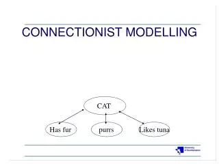
1 0 Inputs 0 Output T McCulloch & Pitts (1943, 1947) The McCulloch & Pitts representation of the “essential” neuron was that it was a logic gate (here an AND gate) The real neuron was far, far more complex, but they felt that they had captured its essence. Neurons were the biological equivalent of logic gates. Conclusion: Collections of neurons, appropriately wired together, can do logical calculus. Cognition is just a complex logical calculus.
Hebb (1949)Connecting changes in neurons to cognition Hebb asked: What changes at the neuronal level might make possible our acquisition of high-level (semantic) information? His answer: Learning rule of synaptic reinforcement (Hebbian learning). When neuron A fires and is followed immediately by the firing of neuron B, the synapse between the two neurons is strengthened, i.e., the next time A fires, it will be easier for B to fire.
High level models of human cognition and behavior Neuronal population coding models Low-level models of single neurons Even lower-level models of synapses and ion channels The HebbianGap Connecting neural function to behavior
Cell assemblies:Closing the Hebbian Gap Cell assemblies at the neuronal level give rise to categories at the semantic level. The formation of cell assemblies involves • persistence of activity without external input. Cell assemblies can overlap. e.g., the cell assembly associated with “dog” will overlap with those associated with “wolf”, “cat”, etc. • recruitment: creation of a new cell assembly (via Hebbian learning) corresponding to a new concept • fractionation: creation of new cell assemblies from an old one, corresponding to the refinement of a concept.
A Hebbian Cell Assembly By means of the Hebbian Learning Rule, a circuit of continuously firing neurons could be learned by the network. The continuing activation in this cell assembly does not require external input. The activation of the neurons in this circuit would correspond to the perception of a concept.
A Cell Assembly Input from the environment
A Cell Assembly Input from the environment
A Cell Assembly Input from the environment
A Cell Assembly Input from the environment
A Cell Assembly Notice that the input from the environment is gone...
Rochester, Holland, Haibt, & Duda (1956) • First real simulation that attempted to implement the principles outlined by Hebb in real computer hardware • Attempted to simulate the emergence of cell assemblies in a small network of 69 neurons. They found that everything became active in their network. • They decided that they needed to include inhibitory synapses. (Hebb only discussed excitatory synapses). This worked and cell assemblies did, indeed, form. • Probably the earliest example in neural network modeling of a network which made a prediction (i.e., inhibitory synapses are needed to form cell assemblies), that was later confirmed in real brain circuitry.
Rosenblatt (1958, 1962): The Perceptron • Rosenblatt’s perceptron could learn to associate inputs with outputs. • He believed this was how the visual system learned to associate low-level visual input with higher level concepts. • He introduced a learning rule (weight-change algorithm) that allowed the perceptron to learn associations.
The elementary perceptron Consists of: • two layers of nodes (one layer of weights) • only feedforward connections • a threshold function on each output unit • a linear summation of the weights times inputs
desired output (“teacher”) t y actual output Threshold = T w w 1 2 x x 1 2 The perceptron (Widrow-Hoff) learning rule (weight-change rule) is: where is the learning constant,
This perceptron learns to associate the visual input of two crossed straight lines with the character “X”. In other words, the output of the network will be the character “X”.
Generalization The real image in the world is degraded, but if the network has already learned to correctly identify the original complete “X”, it will recognize the degraded X as being an “X”.
But not this: This: Y X Y Y Y X X Y Y X X Y Y X Y Y X Y X X X Y X X Fundamental limitations of the perceptron Minsky & Papert (1969) showed that the Rosenblatt two-layer perceptron had some fundamental limitations: They could only classify linearly separable sets.
Input Output 0 0 0 0 1 1 1 0 1 1 1 0 The (infamous) XOR problem • Minsky and Papert showed there were a number of extremely simple patterns that no perceptron could learn, including a logic function XOR. • Since cognition supposedly required elementary logical operations, this severely weakened the perceptron’s claim to be able to do general cognition. XOR There is no set of weights w1 and w2 and a threshold T, such that the perceptron below can learn the above XOR function.
desired output (“teacher”) t y actual output Threshold = T w w 1 2 x x 1 2 The activation arriving at the output node is . If then we output 1, otherwise 0. Butis a straight line if we consider x1 and x2 to be the axis of a coordinate system.
x2 (1,1) (0,1) 0 1 x1 (0,0) (1,0) NO! No values of w1, w2, and T will form a straight line w1x1 + w2x2 = T with (0,1) and (1,0) on one side and (0,0) and (1,1) on the other.
x2 (1,1) (0,1) 0 1 x1 (0,0) (1,0) NO! No values of w1, w2, and T will form a straight line w1x1 + w2x2 = T with (0,1) and (1,0) on one side and (0,0) and (1,1) on the other.
x2 (1,1) (0,1) 0 1 x1 (0,0) (1,0) NO! No values of w1, w2, and T will form a straight line w1x1 + w2x2 = T with (0,1) and (1,0) on one side and (0,0) and (1,1) on the other.
x2 (1,1) (0,1) 0 1 x1 (0,0) (1,0) NO! No values of w1, w2, and T will form a straight line w1x1 + w2x2 = T with (0,1) and (1,0) on one side and (0,0) and (1,1) on the other.
x2 (1,1) (0,1) 0 1 x1 (0,0) (1,0) NO! No values of w1, w2, and T will form a straight line w1x1 + w2x2 = T with (0,1) and (1,0) on one side and (0,0) and (1,1) on the other.
The Revival of the (Multi-layered) Perceptron:The Connectionist Revolution (1985) and the Statistical Nature of Cognition • Minsky (1967): “Within a generation the problem of creating ‘artificial intelligence’ will be substantially solved.” • Minsky (1982): “The AI problem is one of the hardest ever undertaken by science.” By the early 1980’s Symbolic AI had hit a wall. “Simple” tasks that humans do (almost) effortlessly (face, word, speech recognition, retrieving information from incomplete cues, generalizing, etc) proved to be notoriously hard for symbolic AI.
By the early 1980’s the statistical natureof much of cognition became ever more apparent. Three factors contributed to the revival of the perceptron: • the radical failure of AI to achieve the goals announced in the 1960’s • the growing awareness of the statistical and “fuzzy” nature of cognition • the development of improved perceptrons, capable of overcoming the linear separability problems brought to light by Minsky & Papert.
Advantages of Connectionist Models compared to Symbolic AI • Learning: Specifically designed to learn. • Pattern completion of familiar patterns. • Generalization: Can generalize to novel patterns based on previously learned patterns. • Retrieval with partial information: Can retrieve information in memory based on nearly any attribute of the representation. • Massive parallelism. 100-step processing constraint (Feldman & Balard, 1982) Neural hardware is too slow and too unreliable for sequential models of processing. But we can do very complex processing in a few hundred ms. But transmission across a synapse (~10-6 in.) occurs in about ~1 ms. Thus, complex tasks must be accomplished in no more than a few hundred serial steps, which is impossible. • Graceful degradation: when they are damaged, their performance degrades gradually.
Real Brains and Connectionist Networks Some characteristics of real brains that serve as the basis of ANN design: • Neurons receive input from lots of other neurons. • Massive parallelism: neurons are slow but there are lots of them • Learning involves modifying the strength of synaptic connections. • Neurons communicate with one another via activation or inhibition. • Connections in the brain have a clear geometric and topological structure. • Information is continuously available to the brain. • Graceful degradation of performance in the face of damage and information overload • Control is distributed, not central (i.e., no central executive). • One primary way of understanding what the brain does is relaxation to attractors.
General principles of all connectionist networks • aset of processing units • a state of activation defined over all of the units • an output function (“squashing function”) for each unit: Transforms unit activation into outgoing activation; • a connectivity pattern with two features: • - weights of the connections • - locations of the connections • an activation rule for combining inputs impinging on a unit to produce a total activation for the unit • a learning rule, by which the connectivity pattern is changed. • an environment in which the system operates (i.e., how is the i/o represented and given to/taken from the system)
Knowledge storage and Learning • Knowledge storage: Knowledge is stored exclusively in the pattern of strengths of the connections (weights) between units. The network stores multiple patterns in the SAME set of connections. • Learning: The system learns by automatically adjusting the strengths of these weights as it receives information from its environment. There are no high-level rules programmed into the system. Because all patterns are storedin the same set of connections, generalization, graceful degradation, etc. are relatively easy in connectionist networks. It is also what makes planning, logic, etc. are so hard.
Two major classes of networks • Supervised: Includes all error-driven learning algorithms. The error between the desired output and the actual output determines how to change the weights. This error is gradually decreased by the learning algorithm. • Unsupervised: There is no error feedback signal. The network automatically clusters the input into categories. Example: if the network is presented with 100 patterns, half of which are different kinds of ellipses and half of which are different types of rectangles, it would automatically group these patterns into the two appropriate categories. There is no feedback to tell the network explicitly “this is a rectangle” or “this is an ellipse.”
So, how did they solve the problem of linear separability? ANSWER: • By adding another “hidden” layer to the perceptron between the input and output layers, • introducing a differentiable squashing function and iii) discovering a new learning rule (the “generalized delta rule”)
“Concurrent” learning Learning a series of patterns: If each pattern in the series is learned to criterion (i.e., completely) sequentially, the learning of the new patterns will erase the learning of the previously-learned patterns. This is why concurrent learning must be used. Otherwise, catastrophic forgetting may occur. Concurrent learning - 1st pattern presented to the network, change its weights a little to reduce the error on that pattern; - 2nd pattern, change its weights a little to reduce the error on that pattern; - etc. - last pattern, change its weights a little to reduce the error on that pattern; - REPEAT until the error for all patterns is below criterion 1 epoch
Backpropagation Training of a backpropagation network i) Feedforward activation pass with activation “squashed” at hidden layer. ii) The output is compared with the desired output (= error signal) iii) This error signal is “backpropagated” through the network to change the network’s weights (with gradient descent). iv) When the overall error is below a predefined criterion, learning stops.
...but they also suffer from catastrophic interference. Backpropagation networks: Humans:
... but they have trouble learning sequences. Much of our cognition involves learning sequences of patterns. Standard BP networks are fine for learning input-output patterns, they cannot be used effectively to learn sequences of patterns. Consider the sequence: A B C D E F G H I For this sequence we could train a network to associate the following A B B C C D D E E F F G G H H I If we give the network A as it’s “seed”, it would produce B on output, which we would feed back into the network to produce C on output, and so on. Thus, we could reproduce the original sequence.
But what about context-dependent sequences? But what if the sequence were: A B C D E F C H I Here C is repeated. The technique above would give: A B B C C D D E E F F C C H H I But the network could not learn this sequence since it has no context to distinguish the two different outputs associated with C (for the first occurrence, D; for the second, H).
A “sliding window” solution Consider a “sliding window” solution to provide the context. Instead of having the network learn single-letter inputs, it will learn two-letter inputs, thus: AB C BC D CD E DE F EF G FG H GH I Now the network is fed AB (here, “A” servers as “context” for “B”) as its seed and it can reproduce the sequence with the repeated C without difficulty.But what if we needed more than one letter’s worth of context, as in a sequence like this: A BC D E BC H I Now the network needs another context letter...and so on. Conclusion: The Sliding Window technique doesn’t work in general.
Output units Hidden units copy Input units Context units Elman’s solution (1990) The Simple Recurrent Network
SRN Bilingual language learning(French, 1998; French & Jacquet, 2004) • Input to the SRN: • - Two “micro” languages, Alpha & Beta, 12 words each • An SVO grammar for each language • - Unpredictable language switching Attempted Prediction BOY LIFTS TOY MAN SEES PEN GIRL PUSHES BALL BOY PUSHES BOOK FEMME SOULEVE STYLO FILLE PREND STYLO GARÇON TOUCHE LIVRE FEMME POUSSE BALLON FILLE SOULEVE JOUET WOMAN PUSHES TOY.... (Note: absence of markers between sentences and between languages.) The network tries each time to predict the next element. We do a cluster analysis of its internal (hidden-unit) representations after having seen 20,000 sentences.

![Brief [ briefer , briefest ] ( adjective )](https://cdn1.slideserve.com/2610324/brief-briefer-briefest-adjective-dt.jpg)