Bioinformatics Applications of Machine Learning
460 likes | 725 Views
Bioinformatics Applications of Machine Learning. Brian Parker NICTA Life Sciences. Outline. Bioinformatics/computational biology: data analysis of molecular biology datasets Aims of this lecture: To introduce-

Bioinformatics Applications of Machine Learning
E N D
Presentation Transcript
Bioinformatics Applications of Machine Learning Brian Parker NICTA Life Sciences
Outline Bioinformatics/computational biology: data analysis of molecular biology datasets • Aims of this lecture: To introduce- • Some background molecular biology and biotechnology– e.g. microarrays, expressed sequence tags (EST’s) • Some bioinformatics applications of the machine learning methods covered in the lectures so far, and some of the issues and caveats specific to such datasets.
Overview cont’ Applications- • Unsupervised and supervised classification of expression microarrays • Clustering of EST data and EST sequence alignment and discussion of genomic distance measures
Background molecular biology • Central dogma of molecular biology: DNA-> transcribed-> RNA -> translated -> protein • Protein has certain tertiary structures to carry out function e.g. structural elements, enzymes for metabolic processes, gene regulation etc.
Background molecular biology cont’ • DNA is double-stranded polymer of 4 nucleotides (Adenine(A), Cytosine (C), Guanine (G), Thymine (T)) • A gene is a segment of DNA coding for a protein. • mRNA is single-stranded. • Protein is polymer of 20 amino acids • The genetic code maps from the 4-letter alphabet of DNA to the 20–letter alphabet of protein • Note: Recent extension of central dogma--- noncoding RNAs– not translated into protein and directly regulate expression of other genes
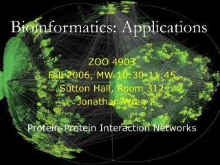
Background molecular biology cont’ These stages lead to several higher-level networks • Gene regulatory networks, pathways • Protein-protein interaction networks • Biochemical networks
Videos • http://www.wehi.edu.au/education/wehi-tv/dna/index.html
High-throughput data analysis • “Omics” = high throughput datasets • Following the central dogma, we have: Genomics from high-throughput sequencing of DNA (genome) Transcriptomics from high-throughput sequencing of RNA and transcribed genome Proteomics from high-throughput analysis of protein Metabolomics from analysis of biochemical metabolites
Microarray technology • Simultaneously measure the expression of 10s of thousands of genes. • Several technologies e.g. Spotted and oligonucleotide arrays (Affymetrix) • Large array of probes designed as a complementary match to the transcript of interest.
Microarray technology • Relies on hybridization– i.e. single-stranded nucleic acids bind to their complement. • mRNA extracted-> reverse transcriptase -> cDNA (biotin-labelled) • -> hybridize to array -> scan image (amount of fluorescence relates to amount of mRNA) • -> convert to expression levels. • Important to normalize arrays to remove variations due to differing lab technique (not covered in this lecture).
Spotted array image Affymetrix array
Microarrays • large p, small n dataset, where n is the number of samples and p is the number of features e.g. 50,000 genes, 100 patient samples is typical • This is the opposite assumption of earlier statistical and machine learning techniques.
Microarrays • Can lead to novel problems: (1) Many techniques assume n <= p e.g. LDA cannot be applied directly as covariance matrix is under-determined and can not be estimated, so feature selection is required. (Even where a method e.g. SVMs can handle the high dimensionality, feature selection is still useful to remove noise genes).
Microarrays (2) Large opportunity for selection bias to occur in feature selection. (3) Large multiple hypothesis correction problem. How to do this without being too conservative? • (Note: we will be talking about expression arrays; there are other array types such as SNP arrays that hybridize with genomic DNA to measure copy number, LOH etc)
Microarray Analysis • 3 broad problems in microarray analysis (Richard Simon): • class discovery (unsupervised classification) (2) class comparison (differential gene expression) (3) class prediction (supervised classification)
Hierarchical clustering– heat map • E.g. Sorlie et. al. (2001) reported several previously unidentified subtypes of breast cancer using clustering. • (Sorlie et al, “Gene expression patterns of breast carcinomas distinguish tumor subclasses with clinical implications”, PNAS)
Filter methods • Specific versus non-specific filtering Non-specific filtering doesn’t use the class labels but removes noise genes of low variance etc. N.B. in clustering, don’t do specific filtering and then cluster!
Specific Filtering • Fold change: simplest method; ratio of expression levels • (but as microarray data is typically log transformed, calculated as difference of means) • t-statistic (one-way ANOVA F-statistic if > 2 samples)– problem is that there often isn’t enough data to estimate variances
Specific Filtering cont’ • Moderated t-statistic. Estimate variance across multiple genes. • Many different versions of moderated variations on the t-test (e.g. regularized t-test of Smyth (2004) (Limma package in Bioconductor), SAM). • They combine a gene-specific variance estimate with an overall predicted variance (e.g. the microarray average) i.e. roughly--
Where is some measure of group difference (e.g. difference of means) is a predicted variance based on all genes, (may be transformed) and is estimated variance based on the particular gene. B is a “shrinkage factor” that ranges from 0 to 1. For B = 1, denominator is effectively constant and so we get the fold change. For B = 0, standard t-test without any shrinkage.
Spike-in experiment results • Experiment with very small spike-in set (6 samples) • (ref. Bioinformatics and Computational Biology Solutions Using R and Bioconductor) • moderated-t better than fold-change better than t-statistic
Embedded and wrapper methods • Wrapper method uses an outer cross-validation– select gene set with smallest loss. • Full combinatorial search is too slow– need to do forward or backward feature selection • Embedded e.g. Recursive feature elimination (RFE) (Guyon and Vapnik). Uses SVM internal weights to rank features– removes worst feature and then iterate. (original paper had a severe selection bias).
Differential gene expression– multiple hypothesis testing • Setting a limit with p-value = 0.05 is too lax due to multiple hypothesis testing. • Doing a multiple hypothesis correction such as Bonferroni correction (multiply p-value by number of genes) is too conservative. In practice, some in-between value may be chosen empirically. • This is controlling family-wise error rate (FWER)– sets the p-value threshold so whole study has a defined false positive rate. For an exploratory study such as differential gene expression, we are willing to accept a higher false positive rate.
False Discovery Rate (FDR) • In this case, what we really want is to specify the proportion of false positives we will accept amongst the gene set we have selected as significant-- the false discovery rate FDR. • Several variants of FDR-- an example is the q-value of Storey and Tibshirani. F = false positives, T = true positives, S = “significant features”
Class Prediction • Can be a classification problem e.g. cancer vs normal or a regression problem, e.g. survival time • Simple methods work well in practice due to small patient numbers. • Dudoit, Fridlyand and Speed compared K-nn, various linear discriminants and CART. • Conclusion: k-nn and DLDA performed best, and ignoring correlation between genes helped: DLDA vs correlated LDA.
Selection bias in microarray studies Because of the high dimensionality and small sample size of microarray data, it is very likely that a random gene will by luck correlate with the class labels. So selecting the best gene set for classification will give an optimistic bias if done outside of the cross-validation loop. It is essential that when using cross-validation, the test set is not used in any way in each fold of the cross validation. This means that all feature selection and (hyper) parameter selection and model selection must be repeated for each fold.
Selection Bias cont’ (From Amboise and McLauclan “Selection bias in gene extraction on the basis of microarray gene-expression data”)
Gene set enrichment analysis (GSEA) • Previous approaches discussed were univariate filter methods, essentially treating each gene independently. • Looking at the overall difference in expression of sets of genes that are known, by other experiments, to be related ,e.g. part of the same pathway or similar gene ontology (GO) annotation, can be a more powerful test to find significant differences.
GSEA • Genes are ranked using a univariate metric • An enrichment score for the gene set is calculated– using a Kologorov-Smirnov-like statistic • The significance level of the enrichment score is computed using a permutation test (where the shuffled labels keep the gene set together). • A FDR is computed to correct for multiple hypothesis testing.
EST analysis • Expressed sequence tags (ESTs) are short, unedited, randomly selected single-pass sequence reads derived from cDNA libraries. Low cost, high throughput. • (cDNA is generated by reverse transcriptase applied to RNA)
EST analysis steps (1) They need to be clustered into longer consensus sequences (unsupervised classification) (2) They can then be sequence aligned against the genome for gene-finding etc. • These two methods require different genomic sequence distance measures…
Similarity measures for genomic sequences • Most data analysis methods use some underlying measure of similarity or distance between samples either explicity or implicitly and this is a major determinant of their performance • e.g. the hierarchical clustering discussed in previous lectures typically has a (dis)similarity matrix passed into the function so that the particular similarity measure used is decoupled from the clustering algorithm
Similarity measures for genomic sequences This idea can be generalized to supervised classification and other data analysis– even when the similarity measure is implicit, it can often be algebraically manipulated to make it explicit (and in this case is the measure is typically a dot product--- generalized by kernel methods to be discussed in later lectures)
Similarity measures for genomic sequences So, it is important to generate good similarity measures between genomic sequences. Two broad classes: Alignment methods and Alignment-free methods
Alignment methods • Model insertions/deletions and substitutions– a form of edit distance • Needleman-Wunsch– global alignment • Based on dynamic programming • Smith-Waterman– local alignment (includes only best-matching high-scoring regions) • BLAST uses a non-alignment-based heuristic to quickly rule out bad matches • Used for sequence alignment and database searching.
Alignment-free methods • Alignment-based distance measures assume conservation of contiguity between homologous segments • Not always the case e.g. ESTs from different splice variants or genome shuffling.
Alignment-free methods • Based on comparing word frequencies • D2 statistic = number of k-word matches between two sequences. • Can be shown to be an inner product of word-count vectors. • Useful for EST clustering
Other areas of bioinformatics • Several other areas of bioinformatics not covered here which also use machine learning techniques • Protein secondary and tertiary structure and motif finding • De novo gene prediction by matching known promoter and coding sequence features.