Download
1 / 34
340 likes | 480 Views
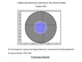
A Mesh-less method for solutions of the Stefan Problem. Vaughan Voller. If A man knows he is going to be hanged tomorrow it concentrates the mind wonderfully— Dr Samuel Johnson 1709-1784. Preliminary Results. Essence of a Numerical Solution. Cover Domain with

E N D
A Mesh-less method for solutions of the Stefan Problem Vaughan Voller If A man knows he is going to be hanged tomorrow it concentrates the mind wonderfully— Dr Samuel Johnson 1709-1784 Preliminary Results
Essence of a Numerical Solution • Cover Domain with • Field of NODES with locations xi 2. Unknowns are nodal values of dependent variable 3. By appropriate APPROXIMATIONS of Governing Equation Obtain a SET Of Discrete Algebraic equations That relate the nodal value at P to Values at the neighbors Process is facilitated by DATA Structure of node points P
If Grid is “square” immediate application of Taylor Series Row i Col. j Approximation Process is facilitated by-- DATA Structure of node points P Location of any node point given a Row, Column index The most Straight Forward Is a STRUCTURED GRID OF NODES
Approximation Process is facilitated by-- DATA Structure of node points n A more flexible approach is use Nodes to Define An UNSTRUCTURED MESH OF ELEMENTS 3 In Each Element obtain a Continuous Approximation Use this approximation with governing equation e.g. in CVFEM--use 2 1
---CLOUDS of Near Neighbor Nodes Approximation Process is facilitated by-- DATA Structure of node points The most flexible approach is to have no mesh Very limited restriction on placement of nodes But may have to be inventive In arriving at sound discrete equations
Simplistic Summary Increasing Flexibility GRID---Structure MESH---FEM “CLOUD”---SPH “Poor” approximation Even Less Efficient solution Ax=b — Very Easy to Fit Geometry Easy to adapt More Complex approximation Less Efficient solution Ax=b — Easy to Fit Geometry Could be Difficult to adapt Easy Approximation Efficient solution Ax=b — Difficult to Fit Geometry
Corrective Smooth Particle Method CSPM -related to SPH Chen et al IJNME 1999 P Taylor Series about node P Multiply by Weighting Factor associated with node P
P 2hp 1.5 > a > 0.5 Properties of W Symmetric about point P Finite region of support Differentiable Char. Length multiple of nearest neig. distance r=R/h
Corrective Smooth Particle Method CSPM -related to SPH Chen et al IJNME 1999 P Taylor Series about node P Multiply by Weighting Factor associated with node P Integrate over support similar manipulations for first derivatives
P Weak point --- Corrective Smooth Particle Method CSPM -related to SPH Chen et al IJNME 1999 Integrate numerically Using particles as integration points 2hp 1.5 > a > 0.5 If Rnb is the radial distance to the neighbors of P r=R/h Critical Feature
At time t>=0 apply a fixed temperature T=Ta >Tm to a patch of the boundary so as to cause a melt region that grows with time b.) time t > 0 T=Ta >Tm Liquid T > Tm n Solid T < Tm liquid-solid interface T = Tm Application to The Stefan Problem--- General problem of Interest Initial state Insulated region containing solid at Temperature T; < Tm (melt temp) a.) time t = 0 Solid Ti < Tm Objective track the movement of the melt front Gmelt
Two-Domain Stefan Model g=1 g=0 T=0 n liquid-solid interface T = 0 Governing Equations Assume constant density and specific heat c — but jump in conductivity K. with time scale and space scales Dimensionless temperature And dimensionless grouping , DH-latent heat, St-Stefan number, L dim. Lat. heat Diffusive Interface—Single Domain Phase change occurs smoothly across A “narrow” temperature range
Particular Versions Two Dimension one-dimension s(t) K=0.25 Ti = 0 T= 0.5 T=1 L=1 T=1 Melting of unit cylinder, initially at phase Change temperature. Has analytical solution Solve in Cartesian Check with fine grid FD solution Using radial symmetry
CSPM Solution P 2hp Use CSPM approximation of derivative twice Backward Euler (explicit) in time Data Structure Global Number nodes 1-----n Identify “cloud” of neighbors associated with each node---- make a list of nodes (global numbers) that fall within a radial distance 2hP Can be manipulated into general form
One-D solution Front Movement K = 0.25 T=1 T=-0.5 o o o CSPM Analytical Dt = 0.002 h = 0.033-0.05 Temperature Profile at time t =2.8 Temperature Histories At ref points Plateau at phase change temp. A feature in all fixed grid solutions
Ti = 0 T=1 For the 2-D problem Need to consider a means of placing out points Two Methods
Discretization: Two steps Put points along boundary of domain— with equal arc spacing Make a structured mesh with spacing SPH Nodes are a List i=1 to nbound Then Lay boundary Mesh Over Structure Mesh Add structured points to SPH node List if they are a distance INSIDE boundary
Black Dot: structured mesh point excluded from SPH list Blue Circle: Boundary Polygon Red Circle: structured mesh point Included in SPH list IDEA stolen from Immersed Boundary Methods of Fotis Sotiropoulos Gives a reasonably Well spaced grid Easy to identify “node Clouds” h = Dr
Results Radial Movement of Front with Time Fine grid radial symmetry solution Melt pattern at An intermediate times
Also works when points are “Jostled”
Unstructured Mesh “Patchy” P Delaunay Good Results But sensitive to choice of h
So far very basic calculations But they show promise— Need to look at Adaptivity Lagrangian
Moving Boundaries in Sediment Transport Two Sedimentary Moving Boundary Problems of Interest Shoreline Fans Toes
Examples of Sediment Fans Moving Boundary Badwater Deathvalley 1km How does sediment- basement interface evolve
Melting vs. Shoreline movement An Ocean Basin
Enthalpy Sol. A 2-D Front -Limit of Cliff face Shorefront But Account of Subsidence and relative ocean level land surface shoreline ocean h(x,y,t) x = s(t) G(x,y,t) Solve on fixed grid in plan view bed-rock y Track Boundary by calculating in each cell x y
A 2-D problem Sediment input into an ocean with an evolving trench driven By hinged subsidence
Need to account for Interaction with channels which can avulse
Increasing Flexibility GRID---Structure MESH---FEM “CLOUD”---SPH “Poor” approximation Even Less Efficient solution Ax=b — Very Easy to Fit Geometry Easy to adapt More Complex approximation Less Efficient solution Ax=b — Easy to Fit Geometry Could be Difficult to adapt Easy Approximation Efficient solution Ax=b — Difficult to Fit Geometry