Download
1 / 32
320 likes | 349 Views
Explore the optimum Carrier Sense distance for maximizing wireless network throughput with considerations for MAC overhead, multirate, and multihop transmissions. Analyze interference models, end-to-end throughput, and bidirectional handshaking effects. Evaluate the impact of exposed and hidden nodes on spatial reuse. Discover the trade-offs and complexities involved in setting multiple Carrier Sense distances for diverse transmission rates. Investigate the implications of bidirectional handshaking on packet collisions, receiver blocking, and protocol stability. Gain insights into achieving maximum spatial reuse in multihop flows while minimizing interference.

E N D
Physical Carrier Sensing and Spatial Reuse in Multirate and Multihop Wireless Ad Hoc Networks Hongqiang Zhai and Yuguang Fang Dept of Electrical & Computer Engineering University of Florida Presented by Tae Hyun Kim
Contents • Problem Statement • Analysis for optimum CS distance • Interference models • … • End-to-end throughput • Simulation • Conclusion • Some comments
Problem Statement • To find optimum CS (Carrier Sense) distance that maximizes throughput • Considered factors • MAC overhead (frame headers and IFSs) • Bidirectional handshaking • Multirate – different TX ranges, RX sensitivities and required SINR • Multihop – forwarding, hidden/exposed nodes, and random topology
Analysis for Optimum CS distance • Notations • Two worst case interference models • Multiple CS distances for multiple rates? • Exposed/hidden node problems • Bidirectional handshaking intensifies interference • End-2-end throughput
Notations Payload size Frame header size Fixed-lengthoverhead
Two Interference Models • Worst case of 6 interferers
Two Interference Models (cont.) • Non-overlapping area of each TX • # of concurrent transmissions • Aggregate throughput • Thus, given SINR, we can find optimum CS distance while fixing transmission distance dt
Two Interference Models (cont.) • Optimum CS distance is, • SINR plays major role other than protocol overhead ≈ 10-10 ≈ 10-7
Two Interference Models (cont.) • 6 interferers scenario may be too conservative • Worst case of only ONE strong interferer • Compute dc’using same method • Optimum CS area reduces to 25~89% of 6 interferers • As shorter CS distance may greatly increase spatial reuse, we may be allowed to decrease dc
Multiple CS distances for Multiple Rates? • Optimum X in interference model varies much, given SINR requirement • Fortunately,RX sensitivities vary much, too • Recall
Multiple CS distances for Multiple Rates? • Optimum CS distances and thresholds by 6 interferers model • Single CS distance is sufficient to maximize throughput
Multiple CS distances for Multiple Rates? • We do have more reasons for single CS distance • High complexity to adapt multiple CS distances for multiple rates • Mobility, distance, channel fading, etc. • Multiple CS distances may introduce additional collisions
Exposed/Hidden Nodes • Exposed node problem • Nodes that are unnecessarily shut up • Let’s define interference range • (X-1)dt=dc-dtfrom receiver • Exposed-area ratio • E.g.) By using 6 interferers model,54 Mbps δ=0.24, 0.56 when X=10, 5, γ>3 Exposed area
Exposed/Hidden Nodes (cont.) • Shorter dc could • Alleviate exposed nodes problem • Achieve higher spatial reuse • Have potentially larger hidden nodes • Hidden node problem • A’s TX is not sensed by C • C may interfere TX from A to B • Increase collisions • Large CS distance can reduce hidden nodes
Exposed/Hidden Nodes (cont.) • Summary • Tradeoff between degrees of exposed nodes and hidden nodes
Bidirectional Handshaking • Bidirectional handshaking incurs • Packet collision by immediate ACK • Receiver blocking (permanent link failure) • Packet collision by immediate ACK • After successfully receiving DATA, ACK is transmitted without CS • RTS may mitigate this as following CTS is sent when channel is idle A B C D DATA DATA ACK
Bidirectional Handshaking (cont.) • Receiver blocking • Before transmitting either CTS or DATA, CS is performed • If there is nearby on-going transmission, receiver never replies to RTS • MAC decides that link has been broken A B C D DATA RTS A receiver does not replyas channel is busy
Bidirectional Handshaking (cont.) • Receivers of previous interferers become new interferers closer to yellow receiver • Modified 6 interferers model • Intuitively, larger dc required to prevent interferers from transmitting
Bidirectional Handshaking (cont.) • Compute optimum CS distance, again • For SINR > - 3dB, • Thus,
Bidirectional Handshaking (cont.) • This solution, • Sacrifices spatial reuse • Increases potential exposed nodes • Incurs MAC contention • But, this also reduces • Potential hidden terminals • Packet collision by immediate ACKs • Receiver blocking
Optimum CS distance • Summary of previous observations • Tradeoff between larger and smaller dc • For protocol stability, larger dc might be better • Optimum CS distance is determined by optimum X* • Simulation study will find μ
Multihop flow consideration • End-2-end throughput • Conditions for maximized spatial reuse along the path • Distance between TXs be less than dc • Not corrupting each other’s packet • N – # of hops between nearest concurrent TXs • 1/N – spatial reuse ratio of a multihop flow • Then, throughput upperbound is N=3 A B C D E F Hop distance
Multihop flow consideration (cont.) • Upperbound for one multihop flow throughput • Observations • Higher rate does not necessarily generate higher throughput IF MAC overhead is taken into account
Multihop flow consideration (cont.) • Consider interference from nearby concurrent transmissions in a regular chain topology • Achievable maximum E2E throughput • This is proportional to BDiP ( ) • May not be maximum in general topology (?!) dc' dc'-dt A B C D E F
Simulation • Modified Ns-2: cumulative interference • 150 nodes in 1000m x 1000 m area • To obtain “one hop” optimum CS distance • Observations • Maximum throughput when 60<CSth*<70 dBm • For some high rates, CSth* < RXse; starving flows exist • Max throughput can be sustained with some starving flows RX sensitivities for different rates
Simulation (cont.) • Optimum CS distance for multihop flows • Observations • CSth* for single hop does not work well • CSth* ~ 91 dBm (smaller CS distance) • Single CS distance could be optimal • Higher rates do not necessarily generate higher throughput Optimum CSth* CSth < RXse randomly selected 20 TCP connections with 500~600 E2E distance
Conclusion • This paper analyzes impact of CS distance to throughput from various perspectives • Found optimum CS distance • Single CS distance is sufficient • dc* may be less than dc due to conservativeness of 6 interferers model • dc * ~ dc + dt due to bidirectional handshaking • dc * = μ(dc / dt + 1) • dt = dh to get maximum E2E throughput • μ can be found by simulation according to network setup
Comments • Based on simplified interference models and extreme cases • Through analysis no relationships between any factors are drawn – only some intuitions • Ignorance on random access MAC overhead – much larger than frame header and IFSs overhead • Packet with higher rate has more overhead proportion, thus penalizing higher rates • Hard to compute BDiP • Does 801.11 do CS before sending CTS and DATA?? • It does not. Nevertheless, receiver blocking can happen due to virtual CS • If rate is adapted, then single CSth* may not be a good strategy
Multihop flow consideration (cont.) • Worst case model for condition (2) • Equivalent to bidirectional handshaking model • We have, • Bound for one multihop flow throughput
Multihop flow consideration (cont.) • Spatial reuse ratio = Ns-2 default: SINR=10 dB, γ=4 Spatial reuse ratio = 1/3