Download
1 / 21
210 likes | 320 Views
This study presents a comprehensive analysis of the angular distribution and ionization processes in HBr upon multi-photon excitation. Utilizing advanced resonance excitation techniques, we investigate the formation of H* and Br* in the presence of H+ ions and explore the dissociation pathways that reveal insights into angular distribution patterns. The approach involves the determination of alignment parameters and the "b" factor through mass-resolved REMPI spectra. The results contribute to a refined understanding of the photodissociation mechanisms and offer a framework for further research in molecular dynamics.

E N D
HBr, angular distribution analysis E(0) Updated, 24.12.2013
E 4 hn ionization / H+ formation H + + Br* H+ + Br H* + Br* 3 hn dissociation / H* formation H* + Br J´ v´ 2 hn resonance excitation v´,J´ HX** Rydb. H+X-/Ion-pair/V H + Br/Br* J´´ v´´= 0 HX r(HX)
According to https://notendur.hi.is/~agust/rannsoknir/papers/jcp121-11802-04.pdf : 3 hn dissociation / H* formation 2 hn resonance excitation
where Unknown (variable in a fit) Unknown (variables in a fit)
BUT simpler for “non Q branches” (O, S) (i.e. for J´´ ¹ J´): 3 hn dissociation / H* formation 2 hn resonance excitation …. i.e. independent of the R´s https://notendur.hi.is/~agust/rannsoknir/papers/jcp121-11802-04.pdf
An alternativewaytoanalysethe angular distributiondatais by theproceduregivenbyChichininet al.:https://notendur.hi.is/~agust/rannsoknir/papers/jcp125-034310-06.pdf -whichinvolvestheuse of relative intensities of spectral lines IQ/IS and IQ/IO whichcouldbederivedfromour REMPI spectra: H* + Br/Br* ph f HBr** i HBr(Ji)
1. Determine „b“ factor, viamassresolved REMPI spectra (see p: 9 https://notendur.hi.is/~agust/rannsoknir/papers/jcp125-034310-06.pdf ) from, 2. Determinealignment parameter A20 (<=„b“ ) (P: 9, https://notendur.hi.is/~agust/rannsoknir/papers/jcp125-034310-06.pdf) (for Jf = 1) (43) (24) (25)
3. Determine angular distribution (wf(n)) viab –factor (b (f)) determination for„f“(seeslide10): (P:6 (and 9), https://notendur.hi.is/~agust/rannsoknir/papers/jcp125-034310-06.pdf) (30) ;Jf = 1 See: http://mathworld.wolfram.com/LegendrePolynomial.html 4. Determinethe angular distribution for one-photonphotodissociation of theunpolarized „f“ state (i.e. w (n,nph)) from for k = 1 (onephoton), wherew (n) is thephotofragment angular distributionproducedby amultiphotonexcitationviatheintermediatestate (i.e. angular distributionderivedfromour experiments) (see p: 6 in https://notendur.hi.is/~agust/rannsoknir/papers/jcp125-034310-06.pdf ) (1)ph
1. Determine „b“ factor, viamassresolved REMPI spectra (see p: 9 https://notendur.hi.is/~agust/rannsoknir/papers/jcp125-034310-06.pdf ) from, a´ c´ d´ a´´ c´´ d´´ Detailed analysis, see : agust,heima, …./PPT-131219.pptx
https://notendur.hi.is/~agust/rannsoknir/Crete/XLS-131221.xlsxhttps://notendur.hi.is/~agust/rannsoknir/Crete/XLS-131221.xlsx
2. Determinealignment parameter A20 (<=„b“ ) (P: 9, https://notendur.hi.is/~agust/rannsoknir/papers/jcp125-034310-06.pdf) (for Jf = 1) (43) (24) (25)
Alignment parameter A20: http://www.ejournal.unam.mx/rmf/no503/RMF50315.pdf , p:319 A20(Jf=1) A20(max) =+0.5 b=-0.5 parallel. domin. b=1 Perpend. domin. A20(min) = -1 b https://notendur.hi.is/~agust/rannsoknir/Crete/PXP-131222.pxp; Gr0,Lay0 <= https://notendur.hi.is/~agust/rannsoknir/Crete/XLS-131221.xlsx
Alignment parameter A20: http://www.ejournal.unam.mx/rmf/no503/RMF50315.pdf , p:319 A20(Jf) Jf = 11 2 1 A20(max;Jf=1) =+0.5 Our A20values = A20 (b = 1.1; b2 = 1.2) b=-0.5 parallel dominant Jf= 1 2 11 A20(min;Jf=1) = -1 b = 1 Perpendiculardominant b factor https://notendur.hi.is/~agust/rannsoknir/Crete/PXP-131222.pxp; Gr0,Lay0 <= https://notendur.hi.is/~agust/rannsoknir/Crete/XLS-131221.xlsx
f <-<- i transitiondominantlyperpendiculartransition, i.e. S <- P <- S 3. Determine angular distribution (wf(n)) viab –factor (b (f)) determination for„f“(seeslide10): (P:6 (and 9), https://notendur.hi.is/~agust/rannsoknir/papers/jcp125-034310-06.pdf) (30) ;Jf = 1 See: http://mathworld.wolfram.com/LegendrePolynomial.html https://notendur.hi.is/~agust/rannsoknir/Crete/XLS-131221.xlsx
wf(n; Jf =1) q https://notendur.hi.is/~agust/rannsoknir/Crete/PXP-131222.pxp; Gr1,Lay1<= https://notendur.hi.is/~agust/rannsoknir/Crete/XLS-131221.xlsx
J´> 1: https://notendur.hi.is/~agust/rannsoknir/papers/jcp125-034310-06.pdf: i.e.: (https://notendur.hi.is/~agust/rannsoknir/papers/jcp121-11802-04.pdf) -butto a first approximation (?) bL = 0 for L = 4,6,…. ERGO: the angular distributionshownonslide 18 holds for all Jf´s ! -in whichcasethealteration in angular distributionvs. J observed (Slide 2) is duetothephotofragmentationstep(?!)
Nowwhat?!How do wederive w(n,nph) ? (1)ph Howabout a „fittingprocedure“:
i.e. somethinglike: (1) + A ~ Experiment ph f b(ph) f i 0 180 q -for redcoloured parameters unknown => deriveb(ph)