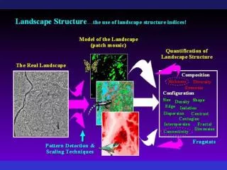
Why Quantify Landscape Pattern?
Why Quantify Landscape Pattern?. Comparison (space & time) Study areas Landscapes Inference Agents of pattern formation Link to ecological processes. Programs for Quantifying Landscape Pattern. FRAGSTATS


Why Quantify Landscape Pattern?
E N D
Presentation Transcript
Why Quantify Landscape Pattern? • Comparison (space & time) • Study areas • Landscapes • Inference • Agents of pattern formation • Link to ecological processes
Programs for Quantifying Landscape Pattern • FRAGSTATS • http://www.umass.edu/landeco/research/fragstats/documents/Metrics/Metrics%20TOC.htm • Patch Analyst • http://flash.lakeheadu.ca/~rrempel/patch/
Quantifying Landscape Pattern • Just because one can measure it, doesn’t mean one should • Does the metric make sense?...biologically relevant? • Avoid correlated metrics • Cover the bases (comp., config., conn.)
Landscape Metrics - Considerations • Selecting Metrics…… • Subset of metrics needed that: • i) explain (capture) variability in pattern • ii) minimize redundancy (i.e., correlation among metrics = multicollinearity) • O’Neill et al. (1988) Indices of landscape pattern. Landscape Ecology 1:153-162 • i) eastern U.S. landscapes differentiated using • dominance • contagion • fractal dimension
Landscape Metrics - Considerations • Selecting Metrics…… • Use species-based metrics • Use Principal Components Analysis (PCA)? • Use Ecologically Scaled Landscape Indices (ESLI; landscape indices, scale of species, and relationship to process)
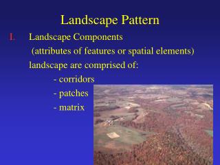
Quantifying Pattern: Corridors • Internal: • Width • Contrast • Env. Gradient • External: • Length • Curvilinearity • Alignment • Env. Gradient • Connectivity (gaps)
Quantifying Pattern: Patches • Levels: • Patch-level • Metrics for indiv. patches • Class-level • Metrics for all patches of given type or class • Zonal or Regional • Metrics pooled over 1 or more classes within subregion of landscape • Landscape-level • Metrics pooled over all patch classes over entire extent
Quantifying Pattern: Patches • Composition: • Variety & abundance of elements • Configuration: • Spatial characteristics & dist’n of elements
Quantifying Pattern: Patches • Composition: • Mean (or mode, median, min, max) • Internal heterogeneity (var, range) • Spatial Characters: • Area (incl. core areas) • Perimeter • Shape
Quantifying Pattern: Landscapes (patch based) • Composition: • Number of patch type • Patch richness • Proportion of each type • Proportion of landscape • Diversity • Shannon’s Diversity Index • Simpson’s Divesity Index • Evenness • Shannon’s Evenness Index • Simpson’s Index
Quantifying Pattern: Patches • Configuration: • Patch Size & Density • Mean patch size • Patch density • Patch size variation • Largest patch index
Patch-Centric vs. Landscape-Centric • Mean – avg patch attribute; for randomly selected patch • Area-weighted mean- avg patch attribute; for a cell selected at random
Patch-Centric vs. Landscape-Centric • Consider relevant perspective…landscape more relevant?...use area-weighted • Look at patch dist’ns…right-skewed = large differences
Quantifying Pattern: Patches • Configuration: • Shape Complexity • Shape Index • Fractal Dimension • Fractals = measure of shape complexity (also amount of edge) • Fractal dimension (d) ranges from 1.0 (simple shapes) to 2.0 (more complex shapes) • ln(A)/ln(P), where A = area, P = perimeter
Quantifying Pattern: Patches • Configuration: • Core Area (interior habitat) • # core areas • Core area density • Core area variation • Mean core area • Core area index
Quantifying Pattern: Patches, Zonal • Configuration: • Isolation / Proximity • Proximity index • Mean nearest neighbor distance
Proximity where, within a user-specified search distance: sk = area of patch k within the search buffer nk = nearest-neighbor distance between the focal patch cell and the nearest cell of patch k
Proximity Index (PXi) = measure of relative isolation of patches; high (absolute) values indicate relative connectedness of patches
Quantifying Pattern • Overlay hexagon grid onto landcover map • Compare bobcat habitat attributes to population of hexagon core areas
Quantifying Pattern • Landscape metrics include: • Composition • (e.g., proportion cover type) • Configuration • (e.g., patch isolation, shape, adjacency) • Connectivity • (e.g., landscape permeability)
Quantifying Pattern & Modeling • Calculate and use Penrose distance to measure similarity between more bobcat & non-bobcat hexagons • Where: • population i represent core areas of radio-collared bobcats • population j represents NLP hexagons • p is the number of landscape variables evaluated • μ is the landscape variable value • k is each observation • V is variance for each landscape variable • after Manly (2005)
Quantifying Pattern & Modeling • Each hexagon in NLP then receives a Penrose Distance (PD) value • Remap NLP using these hexagons • Determine mean PD for bobcat-occupied hexagons Preuss 2005