Download
1 / 32
480 likes | 1.2k Views
An Overview of Tracking Filters. Michael R. Reed EE691/EE692 April 6, 2006 Prepared in partial fulfillment of the requirements for EE691/EE692, with Dr. Emil Jovanov. STOCK MARKET. Tracking Filter Everyday Applications. GPS. WEATHER. Tracking Filter RADAR Applications.

E N D
An Overview of Tracking Filters Michael R. Reed EE691/EE692 April 6, 2006 Prepared in partial fulfillment of the requirements for EE691/EE692, with Dr. Emil Jovanov
STOCK MARKET Tracking Filter Everyday Applications GPS WEATHER
Tracking Filter RADAR Applications • Tracking filter information is used to: • Steer the antenna. • Predict intercept points. • Determine guidance laws for missile commands.
Agenda • General target tracking background • Constant Gain Filters • a-b Filter • a-b-g Filter • Kalman Filter • Simulation Results • Conclusion • 2
Angle Error Generation (Monopulse Beam Patterns) Simultaneous Overlapping and “Squinted” Beams form two Instantaneous Angle Observations True Target position qtgt Beam 1 Beam 2 Angle Q-s qs “Squint “ Angles of the two Beams
a-b Filter Background • Developed in the mid fifties • 2nd order filter • Implies that we can track a constant velocity target with zero error. • Derived from Kalman filter with the following assumptions: • Data rate is constant • Measurement errors are constant • Measurement errors in the different coordinates are independent at each update, i.e. no coupling.
Alpha-Beta Filter error
Coefficient Selection • Benedict Bordner • Kalata • CWTN • Least-Squares
Coefficient Selection Must compromise between the conflicting requirements of good noise smoothing, or narrow bandwidth, and of good transient capability, or wide bandwidth.
Frequency Analysis • Transfer Functions • Filter Bandwidth
Disadvantages • Constant Lag • Inability to handle a maneuvering target • Unable to Vary Update Rate
a-b-g Filter Background • Developed in the mid fifties • 3rd order filter • Implies that we can track a constant acceleration target with zero error • Natural extension of the a-b filter
Alpha-Beta-Gamma Filter error
Coefficient Selection • Neals Simpson
Disadvantages • Tracks a constant velocity target less effectively than the a-b filter • Inability to handle a maneuvering target • Unable to Vary Update Rate
Kalman FilterBackground • Developed by Swerling/Kalman/Bucy • Originally developed for spacecraft navigation for the Apollo space program • Dynamically computes optimum weighting coefficients at each update interval
Kalman Filter … in words • Find forecast position and velocity of target • Find its uncertainty • Use uncertainty of forecast and measurement to calculate filter gain • Find smoothed position and velocity • Find uncertainty in smoothed position and velocity
Coefficient Selection Optimum Kalman Gains
Enter prior estimate and its error covariance Compute Kalman Gain Update Estimate with Measurement & Update State Matrix Compute Error Covariance for Updated Position Project Ahead
Simulation Results Mean a-b Residuals = 0.0531 Mean a-b-g Residuals = 0.0467 Mean Kalman Residuals = 0.0115
REFERENCES Benedict, R. T., & Bordner, G. W. (1962). Synthesis of an optimal set of radar track-while scan smoothing equations. IRE Transactions on Automatic Control, AC-7, 27-32.Ekstrand, B. (2001). Poles and zeros of a-b and a-b-g tracking filters. IEE Proceedings Control Theory Applications, 148, 370-376.Gray, J. E., Smith-Carroll, A. S., & Murray, W. J. (2004). What do filter coefficient relationships mean? Proceedings of the Thirty-Sixth Southeastern Symposium on Systems Theory (pp. 36-40). Dahlgren, VA: Naval Surfare Warfare Center.Gray, J. E., & Murray, W. (1991). The response of the transfer function of an alpha-beta filter to various measurement models. Proceedings of the Twenty-Third Southeastern Symposium on Systems Theory (pp. 389-393). Dahlgren, VA: Naval Surfare Warfare Center.Hovanessian, S.A. (1973). Radar detection and tracking systems. Australia: Artech House, Inc. Kalata, P. R. (1984). The tracking index: A generalized parameter for a-b and a-b-g target trackers. IEEE Transactions on Aerospace and Electronics Systems, AES-20, 174-182.
Munu, M., Harrison, I., & Woolfson, M. S. (1992) Comparison of the Kalman and ab filters for the tracking of targets using phased array radar. Radar 92 International Conference, 196-199.Quigley, A. L. C. (1978). Development of a simple adaptive target tracking filter and predictor for fire control applications. Proceedings of the Tenth Southeastern Symposium on Systems Theory (pp. 1-113). Dahlgren, VA: Naval Surfare Warfare Center.Sklansky, J. (1957, June). Optimizing the dynamic parameter of a track- while-scan system. RCA Laboratories,Princeton, NJ: Author.Skolnik, M. (2001). Introduction to Radar Systems (3rd ed). New York: McGraw Hill.Tenne, D., & Singh, T. (n.d.). Optimal design of a-b-(g) filters. Tenne, D., & Singh, T. (1999). Analysis of a-b-g filters. Proceedings of the IEEE International Conference on Control Applications, USA, (pp. 1342-1347). Range tracking. (2004). Sydney, Australia: University of Sydney, Australian Centre for Field Robotics. REFERENCES (cont.)