Class 2 Quantum mechanics-IB

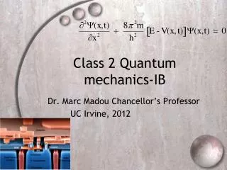
1. Class 2 Quantum mechanics-IB Dr. Marc Madou Chancellor’s Professor UC Irvine, 2012

2. Contents • Time Independent SE or TISE • Applying Schrödinger’s Equation: • Particles in a Large (Infinite) Solid • Particles in a Finite Solid • Quantum Wells (1D confinement)-DOS • Quantum Wires (2D confinement)-DOS • Quantum Dots (3D confinement)-DOS • Tunneling • Harmonic Well • Central Force

3. Time Independent SE or TISE • In the case V(x, t) is independent of time, the SE can be converted into a time independent SE (TISE). Hence we obtain the time independent form of the Schrödinger’s equation as: • Solving this equation, say for an electron acted upon by a fixed nucleus, we will see that this results in standing waves. • The more general Schrödinger equation does feature a time dependent potential V=V(x,t) and must be used for example when trying to find the wave function of say an atom in a oscillating magnetic field or other time-dependent phenomena such as photon emission and absorption.

4. Applying Schrödinger’s Equation:Particles in a Large (Infinite) Solid • For free electrons in an infinitely large 3D piece of metal the allowed electron states are solutions of an expanded version of the Schrödinger equation : • For electrons swarming around freely in this infinite metal, the potential energy V(r) is zero inside the conductor and the solutions inside the metal are plane waves moving in the direction of r: where r is any vector in real space and k is any wave vector. As with a freely moving particle, normalization is impossible as the wave extends to infinity.

5. Plotting the energy E versus the wave number kx for a free electron gas leads to a parabolic dispersion relation. From classical theory we could not appreciate the occurrence of long electronic mean free paths, indeed Drude used the interatomic distance “a” for the mean free path . But from experiments with very pure materials and at low temperatures it is clear the mean free path may be much longer, actually it may be as long as 108 or 109 interatomic spacings or more than 1 cm. The quantum physics answer is that the conduction electrons are not deflected by ion cores arranged in a periodic lattice because matter waves propagate freely through a periodic structure just as predicted by: Confining electrons by limiting their propagation in certain directions in a crystal introduces a varying V(r) in the Schrödinger’s equation and this may lead to an electronic band gap. Applying Schrödinger’s Equation:Particles in a Large (Infinite) Solid

6. Applying Schrödinger’s Equation:Particles in a Finite Solid • Discrete energy levels inevitably arise whenever a small particle such as a photon or electron is confined to a region in space. • Sommerfeld, in 1928, was the first to show this. He adopted Drude’s free electron gas (FEG) and added the restriction that the electrons must behave in accordance with the rules of quantum mechanics (e.g., only 2 electrons per energy level) or he defined a Fermi gas. • In his Fermi gas, electrons are free, except for their confinement within a cubic piece of crystalline conductor with a finite volume of V =L3 and they follow Fermi-Dirac statistics instead of Maxwell-Boltzmann rules.

7. Applying Schrödinger’s Equation:Particles in a Finite Periodic Solid • Outside the 3D cube of solid the potential V(x)= and the wave function  is zero anywhere outside the solid. This situation applies, for example, to totally free electrons in a metal where the ion cores do not influence their movement. Sommerfeld actually assumed that V(x) outside the conductor equaled the work function . • Now let’s introduce periodicity e.g. a repeating cube with side L. The choice of a cube shape with side L is a matter of mathematical convenience. The value L is set by the Born and von Karman’s periodic boundary condition, i.e., that the wave functions must obey the following rule: (x+L, y+L, z+L)=(x,y,z) • Setting such a periodic boundary condition ensures that the free-electron form of the wave function is NOT modified by the shape of the conductor or its boundary. This can be interpreted as follows: an electron coming to the surface is not reflected back in, but reenters the metal piece from the opposite surface. This excludes the surfaces from playing any role in transport phenomena.

8. Applying Schrödinger’s Equation:Particles in a Finite Periodic Solid with Varying Vr • Besides periodicity we also introduce V( r ) ≠ 0. The electrons are not totally free anymore ! They feel the ion cores. • Energy versus wave number for motion of an electron in a one-dimensional periodic potential. The range of allowed k values goes from –π/a to + π/a corresponding to the first Brillouin zone for this system. Similarly, the second Brillouin zone consists of two parts; on extending from π/a to 2π/a, and another part extending between -π/a and -2π/a. This representation is called the extended zone scheme. Deviations from free electrons parabola are easily identified.Where a is the lattice constant.

9. Applying Schrödinger’s Equation:Quantum Wells (1D confinement) • Outside the well and  = 0 for For the Schrödinger equation inside the material (0 <x < L) we write:

10. Applying Schrödinger’s Equation:Quantum Wells (1D confinement) • At the lowest energy (n=1), the ground state, the energy remains finite despite the fact that V=0 inside the region. According to quantum mechanics an electron cannot be inside the box and have zero energy. This is called the zero-point energy an important consequence of the Heisenberg principle.

11. Applying Schrödinger’s Equation:Quantum Wells (1D confinement) • For the same value of quantum number n, the energy is inversely proportional to the mass of the particle and to the square of the length of the box. For a heavier particle and a larger box, the energy levels become more closely spaced. Only when mL2 is of the same order as , do quantized energy levels become important in experimental measurements (with L = 1nm, ). With a 1 cm3 piece of metal (instead of 1nm3), the energy levels become so closely spaced that they seem to be continuous , in other words the quantum mechanics formula gives the classical result for dimension such that meL2 >> Zhores Alferov (Left) and Herbert Kroemer (Right). Nobel Prize in Physics 2000.

12. Applying Schrödinger’s Equation:Quantum Wells (1D confinement) • QWs developed in the early 1970s and constituted the first lower dimensional hetero-structures. The foremost advantage of such a design involves their improved optical properties. • In a quantum well there are no allowed electron states at the very lowest energies (an electron in a box with energy = 0 does not exist) but there are many more available states (higher DOS) in the lowest conduction state so that many more electrons can be accommodated. Similarly, the top of the valence band has plenty more states available for holes. This means that it is possible for many more holes and electrons to combine and produce photons with identical energy for enhanced probability of stimulated emission (lasing)

13. DOS-Bulk Materials • We calculate for the density of states for a parabolic band in a bulk material (3 degrees of freedom) as:

14. DOS-Quantum Well • The density of states function (DOS) for a quantum well is different from that of a 3D solid. The solid black curve is that for free electrons in all 3 dimensions. The bottom of the quantum well is at energy Eg but the first level is at E0. This causes a blue shift. • There are many more states at E0 than at Eg.This makes, for example, for a better laser. • To calculate the current density for a 2D electron gas at a particular temperature we first calculate the value for n(E)2D at T > 0.The function n(E)2D for a given temperature T (>0) is shown as a red line. In the same graph we also show the Fermi-Dirac function and the DOS function (blue).

15. Applying Schrödinger’s Equation:Quantum Wires (2D confinement) • For a particle in a finite sized, 2-D infinitely deep potential well, we define a wave function similar to the 1-D potential well, but now we obtain x,y) solutions that are defined by 2 quantum numbers one associated with each confined dimension.

16. Applying Schrödinger’s Equation:Quantum Wires (2D confinement) • Compared to the fabrication of quantum wells, the realization of nanoscale quantum wires requires more difficult and precise growth control in the lateral dimension, and, as a result, quantum wire applications are in the development stage only. NEC’s Sumio Iijima

17. DOS-Quantum Wire • Quantum wires again feature a blue shift. • Also the density of states (DOS) (blue) and occupied states (red) for a quantum wire are different than those of a 3D electron gas. The Fermi-Dirac function is f(E) and n(E)1D is the product of f(E) and G(E)1D at T>0.

18. DOS-Quantum Wire • For a quantum wire the resistance or current is found to further simplify to a very simple expression that does not depend on voltage but only on the number of available levels. • The amount of current is dictated only by the number of modes (also called sub-bands or channels) M (EF), that are filled betweenEF(1)andF with each mode contributing 2e2/h or: and : This quantized resistance R has a value of 12.906 k

19. DOS-Quantum Wires • Each of the discrete peaks in the density of states (DOS) is due to the filling of a new lateral sub-band. The peaks in the density of states functions at those energies where the different sub-bands begin to fill are called criticalities or Van Hove singularities. These singularities (sharp peaks) in the density of states function leads to sharp peaks in optical spectra and can also be observed directly with scanning tunneling microscopy (STM). • Singularities again emerge when dk/dE= 0

20. Applying Schrödinger’s Equation:Quantum Dots (3D confinement) • In the early 1980s, Dr. Ekimov discovered quantum dots with his colleague, Dr. Efros, while working at the Ioffe Institute in St. Petersburg (then Leningrad), Russia. This team’s discovery of quantum dots occurred at nearly the same time as Dr. Louis E. Brus a physical chemist then working at AT&T Bell Labs found out how to grow CdSe nano crystals in a controlled manner. Columbia’s Louis Brus

21. Applying Schrödinger’s Equation:Quantum Dots (3D confinement) • The solution of the SE for a square semiconductor quantum dot (3D confinement) with side =L and volume V =L3 is given as:

22. DOS Quantumdot • A quantum dot (QD) is an atom-like state of matter often referred to as an “artificial atom.’ • What is so interesting about a QD is that electrons trapped in them arrange themselves as if they were part of an atom although there is no nucleus for the electrons to surround here. • The type of atom the dot emulates depends on the number of atoms in the well and the geometry of the potential well V(r) that surrounds them.

23. Conclusion Reduced DOS as a Function of Dimensionality • An important consequence of decreasing the dimensionality beyond that of quantum wells and quantum wires is that the density of states (DOS) for quantum dots features an even sharper and yet more discrete DOS. • As a consequence, quantum dot lasers exhibit a yet lower threshold current than lasers based on quantum wire and wells, and because of the more widely separated discrete quantum states they are also less temperature sensitive. • However since the active lasing material volume is very small in quantum wires and dots, a large array of them has to be made to reach a high enough overall intensity. Making quantum wires and dot arrays with a very narrow size distribution to reduce inhomogeneous broadening remains a real manufacturing challenge and as a result only quantum well lasers are commercially mature.

24. Applying Schrödinger’s Equation:Tunneling • Outside the box, in regions I and III, the boundary condition is that V(x) = Vo. These are regions that are “forbidden” to classical particles with E < Vo. With E < V0 a classical particle cannot penetrate a barrier region: think about a particle hitting a metal foil and only penetrating the foil if its initial energy is greater than the potential energy it would possess when embedded in the foil and where otherwise it will be reflected. • The solution inside the well is an oscillating wave just as in the case of the well with infinite walls.

25. Applying Schrödinger’s Equation:Tunneling • Defining as : Yields: • In a region with E < V0 there is an immediate effect on the waveform for the particle because, kx is real under these conditions and we can write:

26. Applying Schrödinger’s Equation:Tunneling • We find for the general solution in Region I and III, a wave-function of the form , i.e., a mixture of an increasing and a decreasing exponential function. • With a barrier that is infinitely thick we can see that the increasing exponential must be ruled out as it conflicts with the Born interpretation because it would imply an infinite amplitude. Therefore in a barrier region the wave-function must simply be the decaying exponential . The important point being that a particle may be found inside a classically forbidden region (Region I and III).

27. Applying Schrödinger’s Equation:Tunneling • The exponential decay of the wave function inside the barrier is given as: • If the barrier is narrow enough (L) there will be a finite probability P of finding the particle on the other side of the barrier. The probability of an electron reaching across barrier L is: where A is a function of energy E and barrier height V0.

28. Applying Schrödinger’s Equation:Tunneling • The tunneling current, picked up by the sharp needle point of an STMis given by: • Where fw(E) is the Fermi-Dirac function, which contains a weighted joint local density of electronic states in the solid surface that is being probed and those states in the needle point.

29. Applying Schrödinger’s Equation:Harmonic Well • The time independent Schrödinger equation (TISE) for a harmonic oscillator is given as:

30. Applying Schrödinger’s Equation:Harmonic Well • As expected from Bohr’s Correspondence principle the higher the quantum numbers the better the quantized oscillator resembles the classical non-quantized oscillator.

31. Applying Schrödinger’s Equation: Central Force • An electron bound to the hydrogen nucleus is an example of a central force system: the force depends on the radial distance between the electron and the nucleus only. • The solutions of the Schrödinger equation with this potential are spherical Bessel functions.

32. Summary SE Applications • Summarizing, the quantization for three of the most important potential profiles leads to the following mathematical solutions of the Schrödinger equation: for the central force we obtain spherical Bessel functions, for an infinite square well potential sines, cosines and exponentials and for an oscillator Hermite polynomials.

33. Quantum Jokes