500
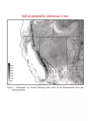
Add all geographic references in text. 3500. Cascade Mountains. 3000. 2500. 2000. 1500. 1000. 500. Sierra Nevada. 3500. 3000. 2500. 2000. 1500. 1000. 500. Figure 1. Topography ( m , shaded following inset scale) of the Intermountain West and adjoining region. a) FULLTER. 3500.

500
E N D
Presentation Transcript
Add all geographic references in text 3500 Cascade Mountains 3000 2500 2000 1500 1000 500 Sierra Nevada 3500 3000 2500 2000 1500 1000 500 Figure 1. Topography (m, shaded following inset scale) of the Intermountain West and adjoining region.
a) FULLTER 3500 3000 2500 2000 1500 1000 500 a) NOSIERRA Figure 2. WRF topography [m, shaded following scale in (a)] for a subset of the (a) FULLTER and (b) NOSIERRA 12-km nested domain.
a) NORTH b) CENTRAL c) SOUTH Figure 3. Outer domain initial 500-hPa geopotential height (black dashed contours, every 120 m) and lowest half-η level potential temperature (gray contours every 3 K) for (a) NORTH, (b) CENTRAL, and (c) SOUTH. Inner domain indicated by inset box. Need to add contour labels. Should be able to do this by hand, perhaps on every other one. I also think the domain Inset position is incorrect in at least one of these. Does the outer domain geographic region shift southward?
Greg-I’ve made some slight adjustments to front/trof positioning here and in subsequent figs Should match Steenburgh et al. (2009) 288 288 288 296 296 296 296 296 296 288 288 288 20 ms-1 10 50 0 45 50 40 -10 30 35 -20 30 10 -30 25 20 -10 -40 15 -50 -30 10 -60 5 -50 -70 a) FULLTER Cloud/Radar 1500 UTC b) NOSIERRA Cloud/Radar 1500 UTC d) NOSIERRA Kinematic (Fw) 1500 UTC c) FULLTER Kinematic (Fw) 1500 UTC e) FULLTER Diabatic (FD) 1500 UTC f) NOSIERRA Diabatic (FD) 1500 UTC Figure 4. WRF-model analyses for 1500 UTC 25 Mar 2006. (a) FULLTER radar reflectivity [dBZ, color shaded according to scale in (a)], cloud-top temperature (°C, grey shaded according to scale in (b)], and geopotential height (solid contours every 10 m). (b) Same as (a) but for NOSIERRA. (c) FULLTER lowest half-η level potential temperature (every 2 K), wind (vector scale at left), and kinematic frontogenesis [K (100 km h)−1, shaded following scale at left]. (d) Same as (c), but for NOSIERRA. (e) Same as (c), but with diabaticfrontogenesis. (f) As in (e) but for NOSIERRA.
288 296 288 296 296 288 296 288 20 ms-1 10 50 0 45 50 40 -10 30 35 -20 30 10 -30 25 20 -10 -40 15 -50 -30 10 -60 5 -50 -70 a) FULLTER Cloud/Radar 1800 UTC b) NOSIERRA Cloud/Radar 1800 UTC d) NOSIERRA Kinematic (Fw) 1800 UTC c) FULLTER Kinematic (Fw) 1800 UTC e) FULLTER Diabatic (FD) 1800 UTC f) NOSIERRA Diabatic (FD) 1800 UTC Figure 5. Same as Fig. 4 except for 1800 UTC 25 Mar 2006.
304 288 296 296 288 288 288 304 304 296 296 304 296 296 20 ms-1 10 50 0 45 50 40 -10 30 35 -20 30 10 -30 25 20 -10 -40 15 -50 -30 10 -60 5 -50 -70 a) FULLTER Cloud/Radar2100 UTC b) NOSIERRA Cloud/Radar2100 UTC d) NOSIERRA Kinematic (Fw) 2100 UTC c) FULLTER Kinematic (Fw) 2100 UTC e) FULLTER Diabatic (FD) 2100 UTC f) NOSIERRA Diabatic (FD) 2100 UTC Figure 6. Same as Fig. 4 except for 2100 UTC 25 Mar 2006.
296 296 288 304 296 288 304 296 288 288 304 304 20 ms-1 10 50 0 45 50 40 -10 30 35 -20 30 10 -30 25 20 -10 -40 15 -50 -30 10 -60 5 -50 -70 a) FULLTER Cloud/Radar 0000 UTC b) NOSIERRA Cloud/Radar 0000 UTC d) NOSIERRA Kinematic (Fw) 0000 UTC c) FULLTER Kinematic (Fw) 0000 UTC c) FULLTER Diabatic (FD) 0000 UTC e) FULLTER Diabatic (FD)0000 UTC d) NOSIERRA Diabatic (FD) 0000 UTC f) NOSIERRA Diabatic (FD)0000 UTC Figure 7. Same as Fig. 4 except for 0000 UTC 26 Mar 2006.
(a) 500 500 500 5 Pa s-1 600 600 600 25 m s-1 Y X 700 700 700 800 800 800 900 900 900 (hPa) (hPa) (hPa) (b) 1000 1000 1000 Y X (c) X Y Figure 3.8. Potential temperature anomaly cross sections. Cross sections of potential temperature (contoured every 2K), and circulation vectors [according to scale in (a)] at 1500 UTC for (a) FULLTERR, (b) NOSIERRA, and (c) FULLTERR-NOSIERRA difference. Location XY shown in Fig. 3.4.
18 UTC Figure 3.9. Skew-T/log pdiagram. Prefrontal skew-T/log pdiagram for FULLTERR (black) and NOSIERRA (gray) at 1800 UTC at locations shown in Fig. 3.5.
a) -2 -2 2 2 0 0 0 0 5 5 2 2 1 1 6 6 4 4 3 3 4 4 11 11 10 10 12 12 7 7 9 9 8 8 4 Group A Group B Group C Group D Group E 4 4 4 15 15 16 16 14 14 17 17 13 13 2 2 19 19 21 21 18 18 20 20 4 4 8 8 6 6 22 22 25 25 23 23 24 24 28 28 29 29 27 27 26 26 0 0 0 30 30 31 31 32 32 0 b) Group A Group B Group C Group D Group E Figure 3.10. Trajectory plots. Backward trajectories ending at 2100 UTC (gray arrow labels denote trajectory number; group A = dark blue, group B = light blue, group C = red, group D = yellow, group E = purple), and potential temperature differences at 2100 UTC (FULLTERR–NOSIERRA; contoured every 2 K) for (a) FULLTERR and (b) NOSIERRA.
0.9 0.7 0.5 0.3 a) 15 2.25 1.75 1.25 0.75 b) Figure 3.11. Analyses for NORTH at 23 h. (a) Lowest η-level baroclinity [shaded according to scale, K (100 km)-1], potential temperature (contoured every 1 K), and wind vectors (m s-1, according to scale). (b) lowest η-level contraction (shaded according to scale, x10-4 s-1), kinematic frontogenesis [every 1 K (100 km)-1 hr-1 starting at 0.25], and wind vectors [as in (a)]. Fronts denoted using conventional frontal symbols, and airstream boundaries denoted by dotted lines.
a) b) Figure 3.12. Analyses for NORTH at 44 h. As in Fig. 3.11.
a) b) Figure 3.13. Analyses for NORTH at 50 h. As in Fig. 3.11.
a) b) Figure 3.14. Analyses for CENTRAL at 23 h. As in Fig. 3.11.
a) b) Figure 3.15. Analyses for CENTRAL at 36 h. As in Fig. 3.11.
a) b) Figure 3.16. Analyses for CENTRAL at 48 h. As in Fig. 3.11.
a) b) Figure 3.17. Analyses for SOUTH at 30 h. As in Fig. 3.11.
a) b) Figure 3.18. Analyses for SOUTH at 45 h. As in Fig. 3.11.
a) b) Figure 3.19. Analyses for SOUTH at 54 h. As in Fig. 3.11.
Greg-I’ve made some slight adjustments to front/trof positioning here and in subsequent figs a) FULLTER 1500 UTC b) NOSIERRA 1500 UTC -30 -20 -10 0 10 -40 -50 -60 -70 5 10 20 25 30 35 40 45 50 15 c) FULLTER 1800 UTC d) NOSIERRA 1800 UTC e) FULLTER 2100 UTC f) NOSIERRA 2100 UTC Figure 4. Simulated radar reflectivity [dBZ, color shaded according to scale in (a)], cloud-top temperature (°C, grey shaded according to scale in (b)], and geopotential height (solid contours every 10 m) for (a) FULLTER at 1500 UTC, (b) NOSIERRA at 1500 UTC, (c) FULLTER at 1800 UTC, (d) NOSIERRA at 1800 UTC, (e) FULLTER at 2100 UTC, and (f) NOSIERRA at 2100 UTC 25 Mar 2006.
288 296 288 288 296 296 20 ms-1 8 7 6 5 4 3 Magnitude for potential temperature gradient? Guessing 10K/100 km – checking with Greg 2 1 b) NOSIERRA Contraction 1500 UTC a) FULLTER Contraction 1500 UTC Figure 5. Lowest half-η level contraction [x10-4 s-1, shaded following scale in (a)], potential temperature (thin contours every 2 K), potential temperature gradient [thick contours every 10 K (100 km)-1], and wind vectors [scale in (a)] at 1500 UTC 25 Mar 2006 from (a) FULLTER and (b) NOSIERRA.
288 296 288 296 20 ms-1 8 7 6 5 4 3 2 1 b) NOSIERRA Contraction 1800 UTC a) FULLTER Contraction 1800 UTC Figure 7. Same as Fig. 5 except for 1800 UTC 25 Mar 2006.
296 288 304 296 288 304 296 20 ms-1 8 7 6 5 4 3 2 1 b) NOSIERRA Contraction 2100 UTC a) FULLTER Contraction 2100 UTC Figure 9. Same as Fig. 5 except for 2100 UTC 25 Mar 2006.
304 288 296 288 296 304 20 ms-1 8 7 6 5 4 3 2 1 b) NOSIERRA Contraction 0000 UTC a) FULLTER Contraction 0000 UTC Figure 11. Same as Fig. 5 except for 0000 UTC 26 Mar 2006.
296 296 288 296 288 296 296 288 288 288 296 288 296 288 288 296 296 288 20 ms-1 50 30 10 -10 -30 -50 b) NOSIERRA Kinematic (Fw) 1500 UTC a) FULLTER Kinematic (Fw) 1500 UTC c) FULLTER Moist (FM) 1500 UTC d) NOSIERRA Moist (FM) 1500 UTC e) FULLTER Boundary Layer (FBL) 1500 UTC e) NOSIERRA Boundary Layer (FBL) 1500 UTC Figure 6. Frontogenesis diagnostics at 1500 UTC 25 Mar 2006 with surface features discussed in text annotated. (a) FULLTER lowest half-η level potential temperature (every 2 K), wind (vector scale at left), and kinematic frontogenesis [K (100 km h)−1, shaded following scale at left]. (b) As in (a), but for NOSIERRA. (c) As in (a), but with moist frontogenesis. (d) As in (d) but for NOSIERRA. (e) As in (a) but with boundary layer frontogenesis. (f) As in (e) but for NOSIERRA.
296 296 288 288 288 288 296 288 296 288 296 296 20 ms-1 50 30 10 -10 -30 -50 b) NOSIERRA Kinematic (Fw) 1800 UTC a) FULLTER Kinematic (Fw) 1800 UTC c) FULLTER Moist (FM) 1800 UTC d) NOSIERRA Moist (FM) 1800 UTC e) FULLTER Boundary Layer (FBL) 1800 UTC e) NOSIERRA Boundary Layer (FBL) 1800 UTC Figure 8. Same as Fig. 6 except for 1800 UTC 25 Mar 2006.
288 304 288 296 296 296 296 288 304 296 304 304 296 296 288 304 296 288 288 304 296 20 ms-1 50 30 10 -10 -30 -50 b) NOSIERRA Kinematic (Fw) 2100 UTC a) FULLTER Kinematic (Fw) 2100 UTC c) FULLTER Moist (FM) 2100 UTC d) NOSIERRA Moist (FM) 2100 UTC e) FULLTER Boundary Layer (FBL) 2100 UTC e) NOSIERRA Boundary Layer (FBL) 2100 UTC Figure 10. Same as Fig. 6 except for 2100 UTC 25 Mar 2006.
296 288 296 288 304 296 288 296 288 304 296 288 296 288 304 304 304 304 20 ms-1 50 30 10 -10 -30 -50 b) NOSIERRA Kinematic (Fw) 0000 UTC a) FULLTER Kinematic (Fw) 0000 UTC c) FULLTER Moist (FM) 0000 UTC d) NOSIERRA Moist (FM) 0000 UTC e) FULLTER Boundary Layer (FBL) 0000 UTC e) NOSIERRA Boundary Layer (FBL) 0000 UTC Figure 12. Same as Fig. 6 except for 0000 UTC 26 Mar 2006.
288 288 296 288 296 296 296 288 296 296 288 288 20 ms-1 50 30 10 -10 -30 -50 b) NOSIERRA Kinematic (Fw) 1500 UTC a) FULLTER Kinematic (Fw) 1500 UTC c) FULLTER Diabatic (FD) 1500 UTC d) NOSIERRA Diabatic (FD) 1500 UTC Figure 6. Frontogenesis diagnostics at 1500 UTC 25 Mar 2006 with surface features discussed in text annotated. (a) FULLTER lowest half-η level potential temperature (every 2 K), wind (vector scale at left), and kinematic frontogenesis [K (100 km h)−1, shaded following scale at left]. (b) As in (a), but for NOSIERRA. (c) As in (a), but with diabaticfrontogenesis. (d) As in (d) but for NOSIERRA.
296 296 288 296 288 296 288 288 20 ms-1 50 30 10 -10 -30 -50 b) NOSIERRA Kinematic (Fw) 1800 UTC a) FULLTER Kinematic (Fw) 1800 UTC c) FULLTER Diabatic (FD) 1800 UTC d) NOSIERRA Diabatic (FD) 1800 UTC Figure 8. Same as Fig. 6 except for 1800 UTC 25 Mar 2006.
20 ms-1 50 30 10 -10 -30 -50 b) NOSIERRA Kinematic (Fw) 2100 UTC a) FULLTER Kinematic (Fw) 2100 UTC c) FULLTER Diabatic (FD) 2100 UTC d) NOSIERRA Diabatic (FD) 2100 UTC FigureX. Same as Fig. X except for 2100 UTC 25 Mar 2006.
20 ms-1 50 30 10 -10 -30 -50 b) NOSIERRA Kinematic (Fw) 0000 UTC a) FULLTER Kinematic (Fw) 0000 UTC c) FULLTER Diabatic (FD) 0000 UTC d) NOSIERRA Diabatic (FD) 0000 UTC FigureX. Same as Fig. X except for 0000 UTC 26 Mar 2006.
1500 1000 500 0 Figure 1. FULLTER topography (contoured every 500-m from light grey to black) and the FULLTERR-NOSIERRA terrain-height difference (m, shaded according to inset scale) Might be better to use all black contours and use contour labels? Perhaps we can live with as is.
Shading here is different than mine Greg used a cint of 5 instead of 4 b) NOSIERRA 1500 UTC Contraction a) FULLTER 1500 UTC Contraction 20 ms-1 3 5 6 1 2 4 7 c) FULLTER 1500 UTC FD d) NOSIERRA 1500 UTC FD Y Y Y Y X X X X -42 -2 2 12 22 32 42 52 -52 -32 -22 -12 Figure 4. (a) Lowest half-η level contraction [x10-4 s-1, shaded according to scale in (a)], baroclinity [dashed contours every 0.5 K (100 km)-1, maxima labeled], kinematic frontogenesis [solid contours every 5 K (100 km)-1 hr-1], and wind vectors [scale in (a)] for FULLTER at 1500 UTC. (b) Same as (a) except for NOSIERRA. (c) Lowest half-ηlevel moist frontogenesis [K (100 km)-1 hr-1, shaded according to scale in (c)], boundary layer frontogenesis [dashed contours every 5 K (100 km)-1 hr-1, , black positive, grey negative], potential temperature (solid contours every 2 K), and wind vectors [as in (a)] for FULLTERR at 1500 UTC. (d) Same as (c) except for NOSIERRA. Surface fronts annotated using conventional frontal symbols, 850-hPa troughs with dashed lines, lowest half-η level airstream boundaries with dotted lines and cross section XY with orange line.
25 8 a) 15 UTC - FULLTERR - Cont., Baro., Kin. Frg. b) 15 UTC - NOSIERRA - Cont., Baro., Kin. Frg. 7 6 5 4 3 2 1 0 c) 15 UTC - FULLTERR - DiabaticFrg. d) 15 UTC - NOSIERRA - DiabaticFrg. Y Y Y Y 60 30 10 -2 2 10 30 60 X X X X Figure 3.4. Mesoscalefrontogenesis diagnostics. Lowest η-level contraction [shaded according to scale in (a), x10-4 s-1], baroclinity [dashed contours, every 0.5 K (100 km)-1, maxima labeled], kinematic frontogenesis [solid contours, every 5 K (100 km)-1 hr-1], and wind vectors [according to scale in (a), m s-1] for (a) FULLTERR and (b) NOSIERRA at 1500 UTC. Lowest η-level moist frontogenesis [shaded according to scale in (c), K (100 km)-1 hr-1], boundary layer frontogenesis [dashed contours, black positive, grey negative, every 5 K (100 km)-1 hr-1], potential temperature (solid contours every 2 K), and wind vectors [as in (a)] for (c) FULLTERR and (d) NOSIERRA at hour 15. Surface fronts are annotated using conventional frontal symbols, 850-hPa troughs using dashed lines, and lowest η-level airstream boundaries using dotted lines. Cross section (Fig. 3.8) position XY also shown.
a) 18 UTC - FULLTERR - Cont., Baro., Kin. Frg. b) 18 UTC - NOSIERRA - Cont., Baro., Kin. Frg. d) 18 UTC - NOSIERRA - DiabaticFrg. c) 18 UTC - FULLTERR - DiabaticFrg. 18 UTC Sounding 18 UTC Sounding 18 UTC Sounding 18 UTC Sounding Figure 3.5. Mesoscalefrontogenesis diagnostics. As in Fig. 3.4 but at 1800 UTC. Position of 1800 UTC sounding (Fig. 3.10) also shown.
a) 21 UTC - FULLTERR - Cont., Baro., Kin. Frg. b) 21 UTC - NOSIERRA - Cont., Baro., Kin. Frg. d) 21 UTC - NOSIERRA - DiabaticFrg. c) 21 UTC - FULLTERR - DiabaticFrg. Figure 3.6. Mesoscalefrontogenesis diagnostics. As in Fig. 3.4 but at 2100 UTC.
b) 00 UTC - NOSIERRA - Cont., Baro., Kin. Frg. a) 00 UTC - FULLTERR - Cont., Baro., Kin. Frg. c) 00 UTC - FULLTERR - DiabaticFrg. d) 00 UTC - NOSIERRA - DiabaticFrg. Figure 3.7. Mesoscalefrontogenesis diagnostics. As in Fig. 3.4 but at 0000 UTC 26 Mar.