Download
1 / 32
400 likes | 883 Views
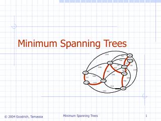
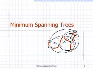
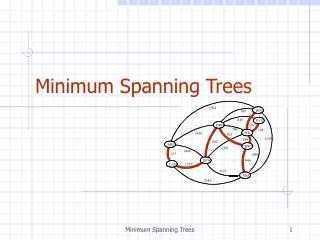
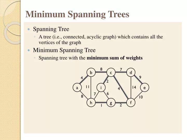
8. 7. b. c. d. 9. 4. 2. a. e. i. 11. 14. 4. 6. 7. 8. 10. h. g. f. 2. 1. Minimum Spanning Trees. Spanning Tree A tree (i.e., connected, acyclic graph) which contains all the vertices of the graph Minimum Spanning Tree Spanning tree with the minimum sum of weights.

E N D
8 7 b c d 9 4 2 a e i 11 14 4 6 7 8 10 h g f 2 1 Minimum Spanning Trees • Spanning Tree • A tree (i.e., connected, acyclic graph) which contains all the vertices of the graph • Minimum Spanning Tree • Spanning tree with the minimum sum of weights
Prim’s Algorithm • Starts from an arbitrary “root”: VA = {a} • At each step: • Find a light edge crossing (VA, V - VA) • Add this edge to set A (The edges in set A always form a single tree) • Repeat until the tree spans all vertices 8 7 b c d 4 9 2 a e i 11 14 4 6 7 8 10 h g f 2 1
8 7 b c d 9 4 2 a e i 11 14 4 6 7 8 10 h g f 2 1 Example 0 Q = {a, b, c, d, e, f, g, h, i} VA = Extract-MIN(Q) a 4 key [b] = 4 [b] = a key [h] = 8 [h] = a 4 8 Q = {b, c, d, e, f, g, h, i} VA = {a} Extract-MIN(Q) b 8 7 b c d 4 9 2 a e i 11 14 4 6 7 8 10 h g f 2 1 8
4 8 8 8 7 7 b b c c d d 8 4 9 9 4 4 2 2 a a e e i i 11 11 14 14 4 4 6 6 7 7 8 8 10 10 h h g g f f 2 2 1 1 8 Q = {c, d, e, f, g, h, i} VA = {a, b} key [c] = 8 [c] = b key [h] = 8 [h] = a - unchanged 8 8 Extract-MIN(Q) c 8 Q = {d, e, f, g, h, i} VA = {a, b, c} key [d] = 7 [d] = c key [f] = 4 [f] = c key [i] = 2 [i] = c 7 4 8 2 Extract-MIN(Q) i 7 2 4
8 8 7 7 8 b b c c d d 4 7 8 4 7 9 9 4 4 2 2 a a e e i i 11 11 14 14 2 4 4 2 6 6 7 7 8 8 10 10 h h g g f f 2 2 1 1 4 8 4 6 7 Q = {d, e, f, g, h} VA = {a, b, c, i} key [h] = 7 [h] = i key [g] = 6 [g] = i 7 4 6 7 Extract-MIN(Q) f 6 7 Q = {d, e, g, h} VA = {a, b, c, i, f} key [g] = 2 [g] = f key [d] = 7 [d] = c unchanged key [e] = 10 [e] = f 7 10 2 7 Extract-MIN(Q) g 10 2
8 8 7 7 b b c c d d 8 8 4 4 7 7 9 9 4 4 2 2 a a e e i i 11 11 14 14 4 4 10 10 2 2 6 6 7 7 8 8 10 10 h h g g f f 2 2 1 1 4 4 2 2 7 1 Q = {d, e, h} VA = {a, b, c, i, f, g} key [h] = 1 [h] = g 7 10 1 Extract-MIN(Q) h 1 Q = {d, e} VA = {a, b, c, i, f, g, h} 7 10 Extract-MIN(Q) d
8 7 b c d 8 4 7 9 4 2 a e i 11 14 4 10 2 6 7 8 10 h g f 2 1 4 2 1 Q = {e} VA = {a, b, c, i, f, g, h, d} key [e] = 9 [e] = d 9 Extract-MIN(Q) e Q = VA = {a, b, c, i, f, g, h, d, e} 9
PRIM(V, E, w, r) % r : starting vertex Total time: O(VlgV+ ElgV) = O(ElgV) • Q ← • for each u V • do key[u] ← ∞ • π[u] ← NIL • INSERT(Q, u) • DECREASE-KEY(Q, r, 0) % key[r] ← 0 • while Q • do u ← EXTRACT-MIN(Q) • for each vAdj[u] • do if v Q and w(u, v) < key[v] • then π[v] ← u • DECREASE-KEY(Q, v, w(u, v)) O(V)if Q is implemented as a min-heap O(lgV) Min-heap operations: O(VlgV) Executed |V| times Takes O(lgV) Executed O(E) times total Constant Takes O(lgV) O(ElgV)
Prim’s Algorithm • Total time: O(ElgV ) • Prim’s algorithm is a “greedy” algorithm • Greedy algorithms find solutions based on a sequence of choices which are “locally” optimal at each step. • Nevertheless, Prim’s greedy strategy produces a globally optimum solution!
We would add edge (c, f) 8 7 b c d 9 4 2 a e i 11 14 4 6 7 8 10 h g f 2 1 Kruskal’s Algorithm • Start with each vertex being its own component • Repeatedly merge two components into one by choosing the lightestedge that connects them • Which components to consider at each iteration? • Scan the set of edges in monotonically increasing order by weight. Choose the smallest edge.
8 7 b c d 9 4 2 a e i 11 14 4 6 7 8 10 h g f 2 1 Example {g, h}, {a}, {b}, {c},{d},{e},{f},{i} {g, h}, {c, i}, {a}, {b}, {d}, {e}, {f} {g, h, f}, {c, i}, {a}, {b}, {d}, {e} {g, h, f}, {c, i}, {a, b}, {d}, {e} {g, h, f, c, i}, {a, b}, {d}, {e} {g, h, f, c, i}, {a, b}, {d}, {e} {g, h, f, c, i, d}, {a, b}, {e} {g, h, f, c, i, d}, {a, b}, {e} {g, h, f, c, i, d, a, b}, {e} {g, h, f, c, i, d, a, b}, {e} {g, h, f, c, i, d, a, b, e} {g, h, f, c, i, d, a, b, e} {g, h, f, c, i, d, a, b, e} {g, h, f, c, i, d, a, b, e} • Add (h, g) • Add (c, i) • Add (g, f) • Add (a, b) • Add (c, f) • Ignore (i, g) • Add (c, d) • Ignore (i, h) • Add (a, h) • Ignore (b, c) • Add (d, e) • Ignore (e, f) • Ignore (b, h) • Ignore (d, f) 1: (h, g) 2: (c, i), (g, f) 4: (a, b), (c, f) 6: (i, g) 7: (c, d), (i, h) 8: (a, h), (b, c) 9: (d, e) 10: (e, f) 11: (b, h) 14: (d, f) {a}, {b}, {c}, {d}, {e}, {f}, {g}, {h},{i}
Operations on Disjoint Data Sets • Kruskal’s Alg. uses Disjoint Data Sets (UNION-FIND : Chapter 21) to determine whether an edge connects vertices in different components • MAKE-SET(u) – creates a new set whose only member is u • FIND-SET(u) – returns a representative element from the set that contains u. It returns the same value for any element in the set • UNION(u, v) – unites the sets that contain u and v, say Su and Sv • E.g.: Su = {r, s, t, u}, Sv= {v, x, y} UNION (u, v) = {r, s, t, u, v, x, y} • We had seen earlier that FIND-SET can be done in O(lgn) or O(1)time and UNION operation can be done in O(1) (see Chapter 21)
KRUSKAL(V, E, w) O(V) • A ← • for each vertex v V • do MAKE-SET(v) • sort E into non-decreasing order by w • for each (u, v) taken from the sorted list • do if FIND-SET(u) FIND-SET(v) • then A ← A {(u, v)} • UNION(u, v) • return A Running time: O(V+ElgE+ElgV) O(ElgE) • Implemented by using the disjoint-set data structure (UNION-FIND) • Kruskal’salgorithm is “greedy” • It produces a globally optimum solution O(ElgE) O(E) O(lgV)
a b c d e f D[.] = 2 0 10 1 Another Example for Prim’s Method 1 f a 2 3 7 S 10 b c 2 a b c d e f a 0 2 7 1 b2 0 10 1 c7 10 0 8 2 d 1 8 0 9 e 2 90 3 f 1 3 0 e 8 1 9 d new D[i] = Min{ D[i], w(k, i)} where k is the newly-selected node and w[.] is the distance between k and i
a b c d e f L [.] = 2 0 10 1 a b c d e f new L [.] = 2 0 8 1 9 1 f a 2 3 7 10 b c 2 a b c d e f a 0 2 7 1 b 2 0 10 1 c 7 10 0 8 2 d 1 8 0 9 e 2 9 0 3 f 1 3 0 e 8 1 9 d new D[i] = Min{ D[i], w(k, i)} where k is the newly-selected node and w[.] is the distance between k and i
ab c d e f L [.] = 2 0 8 1 9 ab c d e f new L [.] = 2 0 7 1 9 1 1 f a 2 3 7 10 b c 2 a b c d e f a 0 2 7 1 b 2 0 10 1 c 7 10 0 8 2 d 1 8 0 9 e 2 9 0 3 f 1 3 0 e 8 1 9 d new D[i] = Min{ D[i], w(k, i)} where k is the newly-selected node and w[.] is the distance between k and i
ab c d e f L [.] = 2 0 7 1 9 1 ab c d e f new L [.] = 2 0 7 1 3 1 1 f a 2 7 3 10 b c 2 a b c d e f a 0 2 7 1 b 2 0 10 1 c 7 10 0 8 2 d 1 8 0 9 e 2 9 0 3 f 1 3 0 e 8 1 9 d
ab c def L [.] = 2 0 7 1 3 1 ab c def new L [.] = 2 0 2 1 3 1 1 f a 2 7 3 10 b c 2 a b c d e f a 0 2 7 1 b 2 0 10 1 c 7 10 0 8 2 d 1 8 0 9 e 2 9 0 3 f 1 3 0 e 8 1 9 d
a b c d e f L [.] = 2 0 2 1 3 1 a b c d e f new L [.] = 2 0 2 1 3 1 1 f a 2 7 3 10 b c 2 a b c d e f a 0 2 7 1 b 2 0 10 1 c 7 10 0 8 2 d 1 8 0 9 e 2 9 0 3 f 1 3 0 e 8 1 9 d Running time: (V2) (array representation) (ElgV) (Min-Heap+Adjacency List) Which one is better?
Greedy MST Methods • Prim’s method is fastest. • O(n2) (worst case) • O(E log n) if a Min Heap is used to keep track of distances of vertices to partially built tree. If e=O(n2), MinHeap is not a good idea! • Kruskal’s uses union-find trees to run in O(E log n) time.
Parallel MST Algorithm (Prim’s) • P processors, n=|V| vertices • Each processor is assigned n/p vertices (Pi gets the set Vi) • Each PE holds the n/p columns of A and n/p elements of d[] array P0 P1 Pi Pp-1 d[.] . . . . . . n/p columns | | | | | | | | | | | | | | | | | | | | | | | | | | | | | | | | | | | | | | | | | | | | | | | | | | | | | | | | | | | | | | | | | | | | | | | | | | | | | | | | | | | | | | | | | | | | | | | | ….. ….. ….. ….. ….. ….. A
Parallel MST Algorithm (Prim’s) 1. Initialize: Vt := {r}; d[k] = for all k (except d[r] = 0) 2. P0 broadcasts selectedV = r using one-to-all broadcast. 3. The PE responsible for "selectedV" marks it as belonging to set Vt. 4. For v = 2 to n=|V| do 5. Each Pi updates d[k] = Min[d[k], w(selectedV, k)] for all k Vi 6. Each Pi computes MIN-di =(minimum d[] value among its unselected elements) 7. PEs perform a "global minimum" using MIN-di values and store the result in P0. Call the winning vertex, selectedV. 8. P0 broadcasts "selectedV" using one-to-all broadcast. 9. The PE responsible for "selectedV" marks it as belonging to set Vt. 10. EndFor
Parallel MST Algorithm (Prim’s) TIME COMPLEXITY ANALYSIS: E=O(n2) then Tseq= n2 (Hypercube) Tpar = n*(n/p) + n*logp computation + communication (Mesh) Tpar = n*(n/p) + n * Sqrt(p) The algorithm is cost-optimalon a hypercube if plogp/n =O(1)
a b c d e f L [.] = 2 0 10 1 Dijkstra’s SSSP Algorithm (adjacency matrix) 1 f a 2 3 7 S 10 b c 2 a b c d e f a 0 2 7 1 b2 0 10 1 c7 10 0 8 2 d 1 8 0 9 e 2 90 3 f 1 3 0 e 8 1 9 d new L[i] = Min{ L[i], L[k] + W[k, i] } where k is the newly-selected intermediate node and W[.] is the distance between k and i
a b c d e f L [.] = 2 0 10 1 a b c d e f new L [.] = 2 0 9 1 10 SSSP cont. 1 f a 2 3 7 10 b c 2 a b c d e f a 0 2 7 1 b 2 0 10 1 c 7 10 0 8 2 d 1 8 0 9 e 2 9 0 3 f 1 3 0 e 8 1 9 d new L[i] = Min{ L[i], L[k] + W[k, i] } where k is the newly-selected intermediate node and W[.] is the distance between k and i
ab c d e f L [.] = 2 0 9 1 10 ab c d e f new L [.] = 2 0 9 1 10 3 1 f a 2 3 7 10 b c 2 a b c d e f a 0 2 7 1 b 2 0 10 1 c 7 10 0 8 2 d 1 8 0 9 e 2 9 0 3 f 1 3 0 e 8 1 9 d new L[i] = Min{ L[i], L[k] + W[k, i] } where k is the newly-selected intermediate node and W[.] is the distance between k and i
ab c d e f L [.] = 2 0 9 1 10 3 ab c d e f new L [.] = 2 0 9 1 6 3 1 f a 2 7 3 10 b c 2 a b c d e f a 0 2 7 1 b 2 0 10 1 c 7 10 0 8 2 d 1 8 0 9 e 2 9 0 3 f 1 3 0 e 8 1 9 d
ab c def L [.] = 2 0 9 1 6 3 ab c def new L [.] = 2 0 8 1 6 3 1 f a 2 7 3 10 b c 2 a b c d e f a 0 2 7 1 b 2 0 10 1 c 7 10 0 8 2 d 1 8 0 9 e 2 9 0 3 f 1 3 0 e 8 1 9 d
a b c d e f L [.] = 2 0 8 1 6 3 a b c d e f new L [.] = 2 0 8 1 6 3 1 f a 2 7 3 10 b c 2 a b c d e f a 0 2 7 1 b 2 0 10 1 c 7 10 0 8 2 d 1 8 0 9 e 2 9 0 3 f 1 3 0 e 8 1 9 d Running time: (V2) (array representation) (ElgV) (Min-Heap+Adjacency List) Which one is better?
Task Partitioning for Parallel SSSP Algorithm • P processors, n=|V| vertices • Each processor is assigned n/p vertices (Pi gets the set Vi) • Each PE holds the n/p columns of A and n/p elements of L[] array as shown below P0 P1 Pi Pp-1 L[.] . . . . . . n/p columns | | | | | | | | | | | | | | | | | | | | | | | | | | | | | | | | | | | | | | | | | | | | | | | | | | | | | | | | | | | | | | | | | | | | | | | | | | | | | | | | | | | | | | | | | | | | | | | | ….. ….. ….. ….. ….. ….. A
Parallel SSSP Algorithm (Dijkstra’s) 1. Initialize: Vt := {r}; L[k] = for all k except L[r] = 0; 2. P0 broadcasts selectedV = r using one-to-all broadcast. 3. The PE responsible for "selectedV" marks it as belonging to set Vt. 4. For v = 2 to n=|V| do 5. Each Pi updates L[k] = Min[ L[k], L(selectedV)+W(selectedV, k) ] for k Vi 6. Each Pi computes MIN-Li = (minimum L[.] value among its unselected elements) 7. PEs perform a "global minimum" using MIN-Li values and result is stored in P0. Call the winning vertex, selectedV. 8. P0 broadcasts "selectedV" and L[selectedV] using one-to-all broadcast. 9. The PE responsible for "selectedV" marks it as belonging to set Vt. 10. EndFor
Parallel SSSP Algorithm (Dijkstra’s) TIME COMPLEXITY ANALYSIS: In the worst-case, Tseq = n2 (Hypercube) Tpar = n*(n/p) + n*logp computation + communication (Mesh) Tpar = n*(n/p) + n * Sqrt(p) The algorithm is cost-optimalon a hypercube if plogp/n = O(1)