Download
1 / 16
170 likes | 332 Views
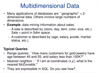
Multidimensional Data. Multidimensional Data. Many applications of databases are "geographic" = 2dimensional data. Others involve large numbers of dimensions. Example : data about sales. A sale is described by (store, day, item, color, size, custName , etc.). Sale = point in 6dim space.

E N D
Multidimensional Data • Many applications of databases are "geographic" = 2dimensional data. Others involve large numbers of dimensions. • Example: data about sales. • A sale is described by (store, day, item, color, size, custName, etc.). • Sale = point in 6dim space. • A customer is described by (custName, age, salary, pcode, maritalstatus, etc.). Typical Queries • Range queries: "How many customers for gold jewelry have age between 45 and 55, and salary less than 100K?" • Nearest neighbor : "If I am at coordinates (a,b), what is the nearest McDonalds." • They are expressible in SQL. Do you see how?
SQL • Range queries: “How many customers for gold jewelry have age between 45 and 55, and salary less than 100K?” SELECT * FROM Customers WHERE age>=45 AND age<=55 AND sal<100; • Nearest neighbor : “If I am at coordinates (a,b), what is the nearest McDonalds.” Suppose we have a relation Points(x,y,name) SELECT * FROM Points p WHERE p.name=‘McDonalds’ AND NOT EXISTS ( SELECT * FROM POINTS q WHERE (q.x-a)*(q.x-a)+(q.y-b)*(q.y-b) < (p.x-a)*(p.x-a)+(p.y-b)*(p.y-b) AND q.name=‘McDonalds’ );
Big Impediment • For these types of queries, there is no clean way to eliminate lots of records that don't meet the condition of the WHERE clause. An Approach for range queries Index on attributes independently. • Intersect pointers in main memory to save disk I/O.
Attempt at using B-trees for MD-queries (example 14.26) • Database = 1,000,000 points evenly distributed in a 1000×1000 square. Stored in 10,000 blocks (100 recs per block) • B-tree secondary indexes on x and on y Range query{(x,y) : 450 x 550, 450 y 550} • 100,000 pointers (i.e. 1,000,000/10) for the x range, and same for y • 10,000 pointers for answer (found by pointer intersection) • Retrieve 10,000 records. If they are stored randomly we need to do 10,000 I/O’s. Add here the cost of B-Trees: • Root of each B-tree in main memory • Suppose leaves have avg. 200 keys 500 disk I/O in each B-tree to get pointer lists 1000 + 2(for intermediate B-tree level) disk I/O’s Total • 11,004 disk I/O’s, more than sequential scan of file = 10,000 I/O’s.
Bitmap Indexes • Suppose we have n tuples. • A bitmap index for a field F is a collection of bit vectors of length n, one vector for each possible value that may appear in the field F. • The vector for value v has 1 in position i if the i-th record has v in field F, and it has 0 there if not. (30, foo) (30, bar) (40, baz) (50, foo) (40, bar) (30, baz) foo 100100 bar 010010 baz 001001
Graphical Picture Customer table. We will index Gender and Rating. Note that this is just a partial list of all the records in the table Two bit strings for the Gender bitmap Five bit strings for the Rating bitmap
Bitmap operations • Bit maps are designed to support partial match and range queries. How? • To identify the records holding a subset of the values from a given dimension, we can do a binary OR on the bitmaps from that dimension. • For example, the OR of bit strings for Age = (20, 21, 22) • To identify the partial matches on a group of dimensions, we can simply perform a binary AND on the OR-ed maps from each dimension. • These operations can be done very quickly since binary operations are natively supported by the CPU.
1 0 1 1 0 1 1 1 OR = 0 1 1 1 1 1 0 0 1 1 0 0 0 0 1 1 1 1 AND = 0 First two records in our fact table are retrieved 0 Bit Map example SELECT * FROM Customer WHERE gender = M AND (rating = 3 OR rating = 5)
Gold-Jewelry Data (25; 60) (45; 60) (50; 75) (50; 100) (50; 120) (70; 110) (85; 140) (30; 260) (25; 400) (45; 350) (50; 275) (60; 260) What would be the bitmap index for age, and the bitmap index for salary? • Suppose we want to find the jewelry buyers with an age in the range 45-55 and a salary in the range 100-200. What do we do?
Compressed Bitmaps • Run length encoding is used to encode sequences or runs of zeros. • Say that we have 20 zeros, then a 1, then 30 more zeros, then another 1. • Naively, we could encode this as the integer pair <20, 30> • This would work. But what's the problem? • On a typical 32-bit machine, an integer uses 32 bits of storage. So our <20, 30> pair uses 64 bits. The original string only had 52!
Run Length Encoding • So we must use a technique that stores our run-lengths as compactly as possible. • Let’s say we have the string 000101 • This is made up of runs with 3 zeros and 1 zero. • In binary, 3 = 11, while 1 is, of course, just 1 • This gives us a compressed representation of 111. • The problem? • How do we decompress this? • We could interpret this as 1-11 or 11-1 or even 1-1-1. • This would give us three different strings after the decompression.
Example: 000000000000010000001 • Here we have two “0” runs of length 13 and 6 • 13 can be represented by 4 bits, 6 requires 3 bits • Run 1: 3 “1” bits + 0 + i → 111 0 1101 • Run 2: 2 “1” bits + 0 + i → 11 0 110 • Final compressed string: 11101101110110 • Compression rate: 14/21 = 0.66 Proper Run Length Encoding • Run of length i has i 0’s followed by a 1. • Let’s say that that we have a run of length i. • Let jbe the number of bits required to represent i. • To define a run, we will use two values: • The “unary” representation of j • A sequence of j – 1 “1” bits followed by a zero (the zero signifies the end of the unary string) • The value i(using j bits) • The special cases of i = 0 and i = 1 use 00 and 01 respectively. Here j=1 so there are no 1 bits (since j-1 =0)
Decoding • Let’s decode 1110110100110110 11101101001011 13 11101101001011 0 11101101001011 3 Our sequence of run lengths is: 13, 0, 3. What’s the bitmap? 0000000000000110001
Summary Pros: • Bitmaps provide efficient storage for low cardinality dimensions. On sparse, high cardinality dimensions, compression can be effective. • Bit operations can support multi-dimensional partial match and range queries Cons: • De-compression requires run-time overhead • Bit operations on large maps and with large dimension counts can be expensive.