
Chapter 12. Option Valuation Using Binomial Model
E N D
Presentation Transcript
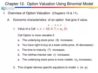
Chapter 12. Option Valuation Using Binomial Model I. Overview of Option Valuation (Chapters 10 & 11). A. Economic characteristics of an option that give it value. + - + + + - 1. Value of a Call = c = f(S, K, T, r, σS, D). Call Option is more valuable if: a. The underlying stock price (S) increases; b. You have right to buy at a lower strike price (K decreases); c. The time to maturity (T) increases; d. The riskfree interest rate (r) increases; e. The underlying stock price is more volatile (σS increases). 2. This chapter derives specific equations to model c (or p).
I.B. Overview – Binomial Option Pricing Model 1. 1-Period Model: C = [ Cu P + Cd (1-P) ] / (1+r) , where P = ((1+r) d) / (u - d), where S0 = today's stock price; follows a Binomial distribution; S0 may by the ratio u with probability P, or by the ratio d with probability (1-P); Cu = value of call if S0; Cd = value of call if S0. 2. 2-Period Model: C = [ CuuP2+ 2Cud P (1-P) + Cdd(1-P)2 ] / (1+r)2 where Cuu= value of call if S0 twice (by u each time); Cdd= value of call if S0 twice (by d each time); Cud= value of call if S0 by u & then by d. 3. N-Period Model: C = S0 B[ a,N,P’ ] - K (1+r)-N B[ a,N,P ]. where a = number of increases out of N trials required for the call to finish in-the-money (S>K); P' = (u / r) P; B[ a,N,P ] = cumulative probability of getting at least a increases out of N trials ( probability that call will finish ITM ). 4. Black / Scholes Option Pricing Model; Limiting case of N-Period Binomial Model. C = S0 N(d1) - K e-rt N(d2); where d1 = [ ln(S0 / K) + (1 + r-.5σS2 ) T ] / σS(T)½ ; and d2 = d1 – σS(T)½ .
II. One-Period Binomial Model A. Example; Assume: 1. S = $50; K = $50, call expires in one year; Tree 2. ST will either increase or decrease by 50% •$75 (i.e., ST = either Su = $75 or Sd = $25, (Cu=$25) where u = 1.5 and d = 0.5); 3. r = .25 $50 • (C = ?) B. Construct riskless “hedge portfolio”: 1. Sell two calls; •$25 2. Buy one share of stock. (Cd=$0) _______________________________________________________ Hedge Portfolio cash flow outcome at end of period today ST= $25 ST = $75 . Sell 2 calls +2c 0 -50 ← must buy 2 shares @ $75; Buy 1 share -50 +25+75and sell @ $50. Total: +2c-50 +25 +25 . [ - - - - - Riskless - - - - - ]
II.C. Solving for the Value of the Call _________________________________________________________ Hedge Portfolio cash flow outcome at end of period today ST = $25 ST = $75 . Sell 2 calls +2c 0 -50 Buy 1 share -50 +25+75 Total: +2c-50 +25 +25 . 1. Note: (investment) = -(flows today) = -2c+50. ←(invest this amount) a. At end of period the payoff is $25 regardless. ← (hedge portfolio) This portfolio should yield the riskless rate (r). (investment) * (1+r) = outcome If c = $15, [-2c+50] * (1.25) = $25 investmt = $20.-2c+50 = $25 / 1.25 [= $20] Borrow $20; -2c = -$30 sell 2 calls, buy 1 sh; c = $15owe $25 (have $25). 2. What if c = $20? Then [-2c+50] * 1.25 $25 Borrow $10; do this. Too high! [-40+50] * 1.25 $25 owe $12.50 (have $25); If c = $20, [$10] * 1.25 $25 keep the rest. investmt = $10. (earn > 1+r with no risk). Do this until c = $15!
II.D. A Generalization 1. Today’s Stock Price = S; Strike = K; Call expires in one year. 2. ST will either increase by u or decrease by d. Tree• $Su (Cu) 3. At expiration, call option will have intrinsic value: Cu = Max { (Su - K), 0 } if S ↑;$S • Cd = Max { (Sd - K), 0 } if S ↓.(C) 4. We wish to know what this call option is worth today (C).• $Sd (Cd) 5. We can solve for this value (C) by constructing a Hedge Portfolio: a. Imagine a portfolio that is long ∆ shares & short 1 call. b. Put another way, Buy Δ shares of stock for each call written. If S ↑ to Su, the value of ∆ shares ↑, & the value of short call (C) ↓; If S ↓to Sd, the value of ∆ shares ↓, & the value of short call (C) ↑. c. We can solve for value of ∆ that makes this hedge portfolio riskless.
II.E. The Hedge Portfolio Hedge Portfolio: Buy Δ shares of stock for each call written. 1. Define: Δ = hedge ratio; the number of shares of stock per call written that makes the payoff independent of S (i.e., riskless); f= c = value of call; fu = cu = value of call if S increases to Su = max { (Su - K), 0 }; fd = cd = value of call if S decreases to Sd = max { (Sd - K), 0 }. In our example, Δ = ½ ; fu= max { 75 - 50, 0 } = $25; fd= $0; f = $15. _____________________________________________________________ 2. Portfolio cash flow outcome at end of pd today ST = SdST = Su . Sell one call: +c -fd-fu Buy Δ shares: -ΔS +ΔSd+ΔSu Total: c-ΔS -fd+ ΔSd -fu+ ΔSu . 3, To be a riskless "hedge portfolio," cash flows at end of period must be same, whether S or : -fd+ ΔSd = -fu+ ΔSu . 4. Solving for Δ, the number of shares per call in the hedge portfolio; Δ = ( fu - fd) / (Su - Sd) = ($25 - $0) / ($75 - $25) = ½. (in our example)
II.E. The Hedge Portfolio Δ = ( fu - fd) / Su - Sd • $Su = $75 (Cu = $25) $S = $50 • (Cu = $15) • $Sd = $25 5. Hedge ratio = dc / dS(Cd = $0) = (Δ option price) / (Δ stock price), as we move between nodes = ($25 - $0) / ($75 - $25) = ½. 6. Define Delta: The ratio of the change in the price of an option to the change in the price of the underlying stock. This is the hedge ratio, Δ; The number of shares we should hold for each call written, in hedge portfolio. Construction of this hedge is called delta hedging (more later).
III. Formula for One-Period Binomial Model A. The hedge portfolio should yield the riskless rate; (riskless investment) * erT = riskless outcome. 1. If we buy Δ shares of stock and sell one call, we have: (initial investment) = (ΔS-c). 2. Thus, (ΔS-c) erT = -fd + ΔSd[ or = -fu + ΔSu] Solving: (c-ΔS) erT = fd- ΔSd c erT = fd - ΔSd + ΔS erT [subst. Δ = (fu- fd) / S(u-d)] c erT = fd - (fu- fd)Sd / S(u-d) + (fu- fd) S erT / S(u-d) c erT = [ fd(u-d) - (fu- fd)d + (fu- fd) erT ] / (u-d) c erT = [ fdu - fdd - fud + fdd + fuerT - fderT ] / (u-d) c erT = [ fu(erT- d) + fd(u - erT) ] / (u-d) c erT = [ fu(erT - d)/(u-d) + fd(u - erT)/(u-d) ] c = [ fup + fd(1 - p) ] e -rT where p = (erT- d) / (u - d)
III. Formula for One-Period Binomial Model c = [ fup + fd(1-p) ] e-rT where p = (erT- d) / (u-d) 3. Interpretation: For a risk-neutral investor (be careful)*, p is probability that stock will increase. Thus, in a risk-neutral world, call value may be interpreted as expected payoff of the option discounted back at the riskfree rate. *** 4. Observe: Many of the factors that affect c appear in this model. C = f ( S, K, T, r, σ, D ); Does S appear in the equation above? K? T? r? ↑ - - - What about σ? What are E(r) & σ2 for binomial distrib? 5. Our Example: (1 + r) = 1.25 (erT) ·$75 S0= $50 u = 1.5 (Cu = $25) K = $50 d = 0.5 $50 · uS0= $75 fu = $25 dS0= $25 fd = $0 ·$25 p = ( erT- d) / ( u - d)(Cd = $0) (1.25 - .5) / (1.5 - .5) = .75 ; (1 - p) = .25 c = [ fu (p) + fd(1 - p) ] e-rT c = [ $25 (.75) + $0 (.25) ] / 1.25 = $18.75 / 1.25 = $15
IV. Risk Neutral Valuation A. Consider the expected return from the stock, when the probability of an up move is assumed to be p. E(ST) = pSu + (1-p)Sd E(ST) = pS(u-d) + Sd [subst. p = (erT- d) / (u-d)] E(ST) = (erT- d) S(u-d) / (u-d) + Sd E(ST) = (erT- d) S + Sd E(ST) = erTS 1. On average the stock price grows at the riskfreerate. 2. Setting the probability of an up movement equal to p is the same as assuming the stock earns the riskfree rate. 3. If investors are risk-neutral, require no compensation for risk, and the expected return on all securities is the riskfreerate.
IV.B. The Risk-Neutral Valuation Principle 1. Any option can be valued on the assumption that the world is risk-neutral. 2. To value an option, can assume: a. expected return on all traded securities is the riskless rate, r; b. the NPV of expected future cash flows can be valued by discounting at r. 3. The prices we get are correct, not just in a risk-neutralworld, but in other worlds as well. 4. Risk-Neutral Valuation works because you can always get a hedge portfolio (that’s riskfree) using options, so arbitrageurs force the option value to behave this way.
V. Two-Period Binomial Model A. Suppose call expires in one year (as before). Can extend framework to two periods by splitting year into two 6-month periods. ● u2S fuu= max{u2S-K,0} ● uS fu= max{uS-K,0} S ●● udS= duS (c) fud= fdu= max{udS-K,0} dS ● fd= max{dS-K,0} d2S ● fdd= max{d2S-K,0} Period 0 Period 1 Period 2 Each branch in Period 2 is like the One-Period Model: fu= [ fuup + fud(1-p) ] e-rΔT fd= [ fudp + fdd(1-p) ] e-rΔT Likewise, for the first period: c = [ fup + fd(1-p) ] e-rΔT where ΔT = 6 months, and r = 6-mo riskfree rate. Can work backward through the Tree.
V.B Formula for Two-Period Binomial Model 1. Each branch in Period 2 can be examined using One-Period Binomial Model: fu = [ fuup + fud(1-p) ] e-rΔT fd = [ fudp + fdd(1-p) ] e-rΔT c = { fup + fd(1-p) } e-rΔT where ΔT = 6 months and r = 6-mo. riskfree rate. 2. Then we can solve for c by substituting for fu and fd above: c = { [ fuup + fud(1-p) ] e -rΔTp + [ fudp + fdd(1-p) ] e -r ΔT (1-p) } e -r ΔT Or: c = { fuup2 + fudp(1-p) + fdu(1-p)p + fdd(1-p)2 } e -r 2ΔT 3. Simply the 1-Period Binomial Model applied twice. a. The same interpretation is maintained: Call value is expected payoff over 2 periods discounted (twice) at (1-pd) riskfree rate. *** 4. Note: Now volatility of S appears directly in formula! Now have all factors! a. σ2 for Binomial distrib. = N p (1-p): Thus, in 2-period model, σ2 = 2 p (1-p).
VI. Determination of u, d, & p The parameters, p, u, & d must be set to give correct values for E(ST) & σ during Δt. Choice of these parameters is critical to the performance of the Binomial Model. To solve for these 3 parameters, we need 3 conditions. A. Given a risk neutral world, stock's expected return is r. E(ST) = S e r Δt= p Su + (1-p) Sd [ S; S disappears ] (1) e r Δt= p u + (1-p) d . This is first condition for u, d, & p. B. Define: σS= instantaneous variance of S, over 1-year interval (annualized). Thus, over time interval Δt, we have standard deviation, σSΔt. The second conditionfor u, d, & p depends on the variance of S over Δt: (2) σSΔt = pu2 + (1-p)d2 - [pu + (1-p)d]2 . C. A third condition is also often imposed: (3) u = 1 / d . This condition makes the tree “recombine;” simplifies computations. D. For small Δt, these 3 conditions are satisfied by: - observe r ; u = e σsqrt (Δt), d = 1 / u, and p = (e r Δt - d) / (u - d). - pick σ & ∆t ; - get u, d, & p.
VII. Working Backward Through the Tree Example: 4 Periods Pick σ & ∆t; Solve for p, u, d, & e r Δt ; Then, given S0, u, & d, fill in the values of S throughout the Tree, & get possible values of c after 4 periods. Next: Apply 1-Period Model to each branch in pd 4; Then work backward through the tree, until you get c today.
VIII. Valuing American Calls & Puts A. Calls. 1. European calls can be valued with Binomial Model. 2. American calls have same value as European calls if no dividend. (C = c) 3. If dividend, can value American calls using modified Binomial model. This valuation is complicated by the American feature. (C ≥ c) Can assume American call will be exercised early if large enough dividend. Binomial tree can be modified to take this into account. B. Puts. 1. Put-Call Parity can be used to price Europeanputs, after you find value of the European call from Binomial Model. 2. Or Europeanputs can be valued directly with Binomial Model, like calls. 3. American puts are different. Will be exercised early if S ↓ (…) (P > p) Must get directly with Binomial trees. Complicated by American feature. Must take into account opportunity to exercise early at each node of tree.
VIII. Valuing American Calls & Puts Example: 5 periods As you work backward through the Tree, Include IF statement at each node in Tree, that compares value from the 1-pd model with the amount ITM. If amount ITM is larger, then exercise at node! Carry this value back through the Tree.
IX. Formula for N-Period Binomial Model c = S * B[ a,N,p’ ] - K e -r N ΔT * B[ a,N,p] where: p = (e r ΔT - d) / (u - d) as before, and p’ = (u / e r ΔT)p ; [ Typically, u > e r ∆t ; so p’ > p. ] a = the lowest number of up moves out of N trials at which the call finishes in-the-month (ITM). B[ a,N,p’ ] = cumulative probability that the number of up moves a out of N trials, where the probability of an up move is p’ (i.e., cumulative probability that option will finish ITM). B[ a,N,p’ ] and B[ a,N,p ] can be found in tables for Binomial distribution, given a, N, & p or p’.
IX. c = S * B[ a,N,p’ ] - K e -r N ΔT * B[ a,N,p] Example: S0 = $50; K = $60; r = .10; u = 1.2; d = .9; N = 10 periods (years). After 1 period, S1 = either S0 u = $60 or S0 d = $45. In this case, after 1 period S1 cannot be > K = $60. Thus the value of a 1-period call at time 0 is $0. Also, ∆ = (cu - cd) / (S0 (u-d)) = 0 = hedge ratio for 1-pd model (= # of shares per call in hedge portfolio). where cu = $0 = max(S0 u - K, 0) = max( $60 - $60, 0); cd = $0 = max( S0 d - K, 0) = max( $45 -$60, 0). There are no values for ∆ that make hedge portfolio for 1 period. However, after 2 pds, call may finish ITM: cuu = max(S0 u2 – K, 0) = max($72 - $60, 0) = $12. With N = 10, have 10 chances for S to rise. To value this call, apply N-Period Model: Call Value = c = S0 B[ a,N,p’ ] - K e -rT B[ a,N,p ], where B[ a,N,p ] = probability of getting ≥ a out of N up moves, given p each period; p = (er ∆t - d) / (u - d) ≈ (1.1-.9) / (1.2-.9) = .67; p’ = pu / er ∆t = (.67 x 1.2) / 1.1 = .73; and where a = min number of up moves out of N needed for call to finish ITM. To find a, solve the following: S0 uadN-a ≥ K or $50 (1.2)a (.9)10-a ≥ $60; a = {1,2,3, …, 10}. Here, it turns out a = 5. If S increases at least 5 out of 10 times, call finishes ITM. Next, see binomial table to find B[a,N,p’] and B[a,N,p]. From this table we have: B[5, 10, .65] = .9051; B[5, 10, .70] = .9527; B[5, 10, .75] = .9803. Interpolating: B[5, 10, .67] = .926 and B[5, 10, .73] = .972 Now we have all the information to solve N-Period Binomial Model for c: Call Value = $50 x (.972) - $60 x (.386) x (.926) = $27.20
c = S * B[ a,N,p’ ] - K e -r N ΔT * B[ a,N,p] Table of Binomial Probabilities n 10 11
X. What if Stock Pays a Dividend? Example: If stock will pay a dividend with NPV = D, then expect S to ↓ by D when paid. The Binomial Tree can be modified to account for the expected decline in S, at the time of the dividend. Note: If S is adjusted down by the amount D, then the Tree does not re-combine following the dividend. This feature makes the analysis somewhat more cumbersome. But this is a simple task for computers.
X. What if Stock Pays a Dividend? Example: If stock index pays a continuous dividend yield, δ, then expect S to ↓ by δ when D is paid. In this case, the Tree does recombine.