Download
1 / 33
340 likes | 418 Views
Explore the mathematical interpretation of generating functions for point charges, electric multipoles, and associated Legendre functions. Learn about the significance of spherical harmonics and understand the mathematical implications of multipole expansions.

E N D
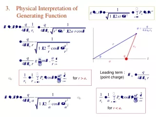
3. Physical Interpretation of Generating Function Leading term : (point charge) forr > a. forr < a.
Expansion of 1 / | r r | Let : either r or r on z-axis
Electric Multipoles Electric dipole : point dipole Leading term :
(Linear) Multipoles Let = 2l-pole potential with center of charge at z = r. Mono ( 20 ) -pole : Di ( 21 ) -pole : Quadru ( 22 ) –pole : ( 2l ) –pole : Quadrupole Mathematica
Multipole Expansion If all charges are on the z-axis & within the interval [zm, zm ] : for r > zm where is the (linear) 2l–pole moment. For a discrete set of charges qiat z = ai.
If one shifts the coord origin to Z. • lis independent of coord, i.e., Z • iff Multipole expansion for a general (r) are done in terms of the spherical harmonics.
4. Associated Legendre Equation Associated Legendre Eq. Let Set Mathematica
Frobenius Series with indicial eqs. or By definition, Mathematica
Series diverges at x = 1 unless terminated. For s = 0 & a1= 0 (even series) : ( l,mboth even or both odd ) Mathematica Fors = 1 & a1=0 (odd series) : (l,mone even & one odd ) Plm = Associated Legendre function
Relation to the Legendre Functions Generalized Leibniz’s rule :
Set Associated Legendre function : ()mis called the Condon-Shortley phase. Including it in Plmmeans Ylmhas it too. Rodrigues formula : Mathematica
Generating Function & Recurrence ( Redundant since Plm is defined only forl |m| 0. ) &
as before
( Redundant since Plm is defined only forl |m|0. ) &
Recurrence Relations for Plm (1) = (15.88) (2) (1) : (3) (3) (2) : (15.89)
Table 15.3 Associated Legendre Functions Using one can generate all Plm (x)s from the Pl (x)s. Mathematica
Example 15.4.1. Recurrence Starting from Pmm (x) no negative powers of (x1)
l = m l = m+k1 E.g., m = 2 :
Parity & Special Values Rodrigues formula : Parity Special Values : Ex.15.4-5
Orthogonality Plm is the eigenfunction for eigenvalue of the Sturm-Liouville problem where Lm is hermitian ( w = 1 ) Alternatively :
No negative powers allowed For p q , let & only j = q ( x = + 1) or j = kq ( x = 1 ) terms can survive
pq: For j > m : For j < m + 1 :
pq: Only j = 2mterm survives
Ex.13.3.3 B(p,q)
For fixed m, polynomials { Ppm (x) } are orthogonal with weight ( 1 x2 )m. Similarly
Example 15.4.2. Current Loop – Magnetic Dipole Biot-Savart law(for A , SI units) : By symmetry : Outside loop : E.g. 3.10.4 Mathematica
For r > a :
For r > a :
on z-axis : or (odd in z)
Biot-Savart law(SI units) : Cartesian coord:
For r > a :