Download
1 / 20
200 likes | 882 Views
Chapter 9 – Production & Cost in the Short Run. Our focus has been on the fact that firm’s attempt to maximize profits. However, so far we have only focused on the revenue side of profits and have ignored costs.

E N D
Chapter 9 – Production & Cost in the Short Run • Our focus has been on the fact that firm’s attempt to maximize profits. However, so far we have only focused on the revenue side of profits and have ignored costs. • Increased globalization of markets has forced firm’s to focus more on productivity and control of costs in order to compete in the international market place.
Short Run versus Long Run • In the short run at least one input is fixed in quantity and cannot be changed. • In the long run all inputs are variable. Thus, even plant size can be changed (capital decisions). • Short run costs will depend on short run production theory and long run costs on long run production theory.
Production Functions • A production function is a relationship(table, graph, or equation) showing the maximum output that can be produced from any specified set of inputs, given the state of technology. • Our production function to allow for graphical efficiency is of the following form: Q = f(L,K)
Technical Efficiency versus Economic Efficiency • Technical efficiency is achieved when output is maximized for any combination of inputs. Thus, any point on the production function is technically efficient. • Economic efficiency is achieved when a given level of output is generated at least cost. • Note a process may be technically efficient and not economically efficient. • Example – building airfields in SE Asia during WWII (price of inputs becomes important n economic efficiency).
Some Definitions • Inputs can be • Fixed – level of usage cannot be changed • Land • Capital • Variable – level of usage can be changed • Labor services • Raw materials
Short Run(SR) Production Function • In SR, recall that time period is such that at least one input is fixed in amount. Thus, the SR production function can be written as K-bar implies a fixed amount of capital.
Production in the Short Run • Use simplest of cases – where output, Q, is a function of a single input, L, Labor. • Total Product is same as output or Q. • Average Product = AP = Q/L • Marginal Product = MP = Change in Q/Change in L
#7, page 349 A Production Function Long run – let both K and L vary Short run – fix K and let L vary
#7, page 349 A Short Run Production Function Short run – fix K at L=2 and let L vary
#7, page 349 A Short Run Production Function: K=2
Law of Diminishing Marginal Product • This is one of the “strictest” laws in economics. • It states that as the number of units of the variable input increases, holding constant all other inputs, a point is eventually reached where marginal product will decline.
Graph of Total, Average, and Marginal Products • See Figure 9.1, page 326. • What happens to curves if the fixed input, K, is increased? • Important points • TP curve must eventually increase at a diminishing rate(law of diminishing marginal productivity). This occurs where slope of TP, which is MP, starts to decline • MP intersects AP at maximum AP. When AP is rising AP > MP. When AP is falling, MP < AP • MP = 0 where TP is max
Economic Costs • Opportunity cost is the value of what firm owners give up to use a resource. It is the sum of explicit(money flows) costs as well as implicit costs(no money flows) • Explicit costs – an out-of-pocket monetary payment for the use of a resource. • Implicit costs – the foregone return the firm’s owners could have received had they used their own resources in their (next best) alternative use.
Normal Profit • Normal Profit is nothing more than implicit cost of using owner supplied resources. • Capital(best alternative use?) • Lease or rental value • Sell and invest proceeds(current market value and not purchase price is relevant) • Owner’s time
Short Run Costs • In SR some inputs are fixed. Thus, these resources must be compensated irrespective of output and lead to some costs being fixed(independent of output). We refer to these as fixed costs, TFC. • Payments for variable inputs are called variable costs, TVC, and these depend on output. • Total Cost = TVC + TFC
Other SR Cost Concepts • Average Fixed Cost = AFC = TFC/Q • Average Variable Cost = AVC = TVC/Q • Average Total Cost = ATC = TC/Q • ATC = AVC+AFC • SR Marginal Cost = SMC = (change in TC or TVC)/change in Q
Relationships among Average and Marginals • ATC, AVC, and SMC all have U-shape with respect to output • AFC continuously declines – “spreading the overhead” • SMC is above(below) ATC when ATC is increasing(decreasing). Same for AVC and SMC relationship. • SMC intersects AVC and ATC at their minimum points respectively.
SR Cost and SR Production – the Linkage • Recall SR production function is Q = f(L) since K is assumed fixed. • Thus, TVC = w * L and TFC = r * K where w = price of labor(wage rate) r = price of capital • So TC = wL + rK
AVC versus AP • Recall AVC = TVC/Q and TVC = wL, so • AVC = wL/Q or AVC = w/(Q/L) = w/APL • Note the significance of this. AVC is related to the wage rate, which for the firm is assumed to be fixed(price-taker) and the average product of labor(APL). • AP curves initially increase as the quantity of labor increases, reach a max , and then decline. Thus, AVC will do the opposite – decrease, reach a minimum, and then increase.
MC versus MP • Note MC is the wage rate, which is assumed fixed) divided by the marginal product of labor. • Thus, as MP rises(falls), MC falls(rises). Also the max of MP is the minimum for MC • See Figure 9.7