Download
1 / 51
510 likes | 647 Views
The multiple causes of summer mesospheric warmings. David E. Siskind (with assistance from J. P. McCormack, D. Drob, M. Stevens and the AIM science team) Space Science Division Naval Research Laboratory. Outline The NASA Aeronomy of Ice in the Mesosphere (AIM) mission

E N D
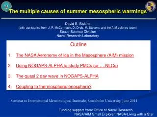
The multiple causes of summer mesospheric warmings David E. Siskind (with assistance from J. P. McCormack, D. Drob, M. Stevens and the AIM science team) Space Science Division Naval Research Laboratory Outline The NASA Aeronomy of Ice in the Mesosphere (AIM) mission Using NOGAPS-ALPHA to study PMCs (or ….NLCs) The quasi 2 day wave in NOGAPS-ALPHA Coupling to thermosphere/ionosphere? Seminar to International Meteorological Institude, Stockholm University, June 2014 Funding support from: Office of Naval Research, NASA/AIM Small Explorer, NASA/Living with a Star
Clouds at the Edge of Space Tom Eklund, July 28, 2001, Valkeakoski, Finland PMC: Polar Mesospheric clouds NLC: noctilucent clouds • Polar summer • ~ 83 km altitude • Water ice and meteoric • smoke crystals • 30 nm to 80 nm size • Coldest spot on Earth • > 50o latitude N and S • First observed in 1885 • Possible connection with with global change (increased humidity from CH4 increases) motivation for AIM/SMEX NH Season: mid-May to mid-August SH Season: mid-November to mid-February
Aeronomy of Ice in the Mesosphere: AIM Cloud Imaging and Particle Size Exp. (CIPS) Solar Occultation For Ice Exp. (SOFIE) Launched in March, 2007. The beginning of the Great Solar Minimum
Current understanding of mesopause variability Gumbel and Karlsson, GRL, 2011 Anticorrelation with radius of OSIRIS PMCs (a proxy for brightness and hence cold temps) (Karlsson et al, GRL, 2007) Winter stratospheric weather drives summer mesospheric weather in opposite hemisphere
Strat temps extended to 2010 Note that 2007 was warm and 2008 was cold
Increasing solar activity ? Early AIM data and teleconnections (July: 07-10) Ice Water Content (g/km2) vsTeleconnection Index TI 2008 2008 2009 2009 2010 2010 2007 2007 Expected to anticorrelate: Increased UV will heat mesosphere and dissociate H2O (Garcia, 1989; Siskind et al, 2005)
Solar Activity begins to increase F107_jul11 = 94 F107_jul12 = 136
2008 2009 2010 2007 The next year……..(mean July F107 went from 68 94) IWC vsTeleconnection Index TI Woops! Wrong direction
The following year……..(July F107 went to 136) Diamonds and squares are two diff. estimates of teleconnection IWC (g/km2) CIPS generally agrees with SOFIE.Certainly no solar cycle decline in 2011-2012!!
High IWC Anomaly Recent enhancements most pronounced for IWC > 150 g km-2 even greater disagreement with SBUV
The total water budget (ice+vapor) Only for the > 200 g/km2 IWC clouds We suggest a 2nd source of water to the high lat mesosphere
Space Traffic Stevens provides answer After some refinement for consistent dates What about this??
Big shuttle launch in 2009 At a local time such that it moved (initially) south From Siskind et al 2003, GRL HRDI wind climatology STS 127 launch, July 15, 2009 Confirmed by MLS observations of the plume (Pumphrey et al., 2011) So we’re consistent: No solar cycle variation, PMC variation due both to interhemispheric coupling modulated by space traffic The 2012 anomaly is interesting because its post-shuttle era
Theory Coupling Fig 8 of E. Becker review: difference fields for cases w/ and w/o SSW MC SSW The temperature deviation at 30 km in winter is correlated with mesopause temp anti correlated with PMC This deviation is used to define a teleconnection index
NOGAPS-ALPHA: a project to lift the lid on the US Navy’s forecast system(Advanced Level Physics High Altitude) Operational NOGAPS, 2000 First stage (2005) final extension (2007) • new hybrid s-p vertical coordinate (to maintain smooth vertical layer thickness profiles over all topography; increased vertical domain), increased vertical resolution • new physics packages (short wave (MUV) heating, prognostic ozone) • non-LTE cooling (Fomichev) extends model to 110-115 km (up to 74 levels) • WACCM gravity wave scheme (Garcia et al., JGR, 2007)
Forecast/Assimilation Cycling Global Spectral Forecast Model 0-10 Day Forecasts 0-9 Hour Forecasts Global 0-100 km observations over next 0-6 hours Xb Xa 6 hourly global 0-100 km analysis fields Data Assimilation System NAVDAS/NAVDAS-AR y
High Altitude Assimilation NAVDAS: NRL Atmospheric Variational Data Assimilation System Top Data Insertion Operationally Top Data Insertion ~1 hPa 0.002 hPa Version 2.2 MLS Temperature Version 1.07 SABER Temperature Water Vapor Ozone Credit: Karl Hoppel: karl.hoppel@nrl.navy.mil
Pattern of Warm anomalies
Summary of High Altitude Analysis Coverage: June 2007 – March 2010, plus Dec 2004/Feb 2005 Dec 2005/Feb 2006 Thus: 3 NH summers and 5 SH summers Altitude range: generally valid up to 0.001 hPa Note, NOGAPS-ALPHA has been superseded by NAVGEM (Hoppel et al., 2013); however, the above analysis remains the only analysis valid up to 90 km
July 2007 minus 2008 temperatures NAVDAS, the data assimilation component of NOGAPS-ALPHA (Eckermann et al., 2009; 3DVar , uses SABER and MLS data)
NOGAPS-ALPHA for 2 NH winters 2008 2006 Temp 80N Zonal Wind 60N Planetary Wave 1, 60N
Planetary wave amplitude: 60S, NAVDAS Jul Aug Sep Oct Planetary waves were enhanced in 2007 relative to 2008.
Interhemispheric Coupling: 3 Steps Standard conditions: NH winter warmer than Trad SH summer colder than Trad Perturbed conditions: 1. SSW warming 2. Mesospheric cooling 2a. Tropical mesospheric warming (“this seesaw is crucial” Becker, 2012) 3. from thermal wind; zonal winds perturbed in SH subtropics which effect GWD in summer B. Karlsson used CMAM to propose step 3 above
Quote from a colleague He or she can accept that it happens but the mechanism sounds like “a Rube Goldberg mechanism”
From Wikipedia: deliberately over-engineered or overdone machine that performs a very simple task in a very complex fashion, usually including a chain reaction(Rube Goldberg, American cartoonist and inventor, 1883-1970) The Self-Operating Napkin Rube Goldberg Mechanism The "Self-Operating Napkin" is activated when soup spoon (A) is raised to mouth, pulling string (B) and thereby jerking ladle (C), which throws cracker (D) past parrot (E). Parrot jumps after cracker and perch (F) tilts, upsetting seeds (G) into pail (H). Extra weight in pail pulls cord (I), which opens and lights automatic cigar lighter (J), setting off skyrocket (K) which causes sickle (L) to cut string (M) and allow pendulum with attached napkin to swing back and forth, thereby wiping chin.
In German For the benefit of Chris Englert and Franz Josef Lubken: such machines are often called "Was-passiert-dann-Maschine" ("What happens next machine") for the German name of similar devices used by Kermit the Frog in the children's TV show Sesame Street.
Solar Cycle Variation of PMCs Data from SBUV (Shettle, Deland et al., JGR 09) One longstanding puzzle is why the effect is greatest at the highest latitude when conditions are closer to threshold at sub-arctic latitudes
Summary of NH variation Teleconnections: Karlsson/Becker mechanism agrees with NOGAPS and with PMC data for the 1st 4 Northern Summers
How does the exhaust get there? First: at 100-110 km, it is consistent with mean flow to summer pole e.g. Figure 1 of Smith et al., 2011, WACCM winds But this is too slow. Needs something to “kick” it- esp. for the single SH observation of Stevens et al (2005, GRL)
Quasi 2 Day waveNiciejewski et al. 2011, JGR Analysis of TIDI winds Wave number 3, 0.5 cycles/day
Q2DW in NOGAPS-ALPHA H2O: Jan 06(McCormack et al., 2009) Direction of propagation Westward propagating Wave 3.
Average for January 2006 Peak v component in MLT, SH mid-latitudes- right where you’d need it for plume transport
Problem: 2006 was unique For 2009, year with biggest SSW ever, bigger than 2006 For 2005, year with cold NH winter Contrary to first impressions, there is no one-to-one link between an SSW and enhancements in Q2DW
And yet…. A link with PMCs? ?? Q2DW in tropical thermosphere responds to mesopause winds? 2006 zonal winds at 98 km (calculated by TIEGCM) were the weakest in all 5 years of NOGAPS-ALPHA Mesopause (p=.002 hPa, 88km) temperatures in NOGAPS-ALPHA for 5 Southern Summers 2005 121 2006 138 Unusually warm mesopause in 2006 2008 124 2009 123 2010 123
2006 already identified as anomalous in PMCs Gumbel and Karlsson find fewest PMCs In OSIRIS in SH summer of 05/06 Teleconnection Index in 2006 is very warm And TI for SH summer of 08/09 is cold Linkage of correlations: fewest PMCs due to warmest mesopause weakest zonal winds at 98 km The weakening of the winds seems to lead the enhancement of a strong Q2DW which extends up into tropical thermosphere (ionospheric dynamo region)
Q2DW in NOGAPS/NAVDAS(Eckermann et al., 2009; 3DVar , uses SABER and MLS data) p=.0013 hPa, 46 S 2006 2005 2010 2008 2009 2005 and 2006 Q2DW enhancements, eddy heat flux and EP flux divergence linked to the temperature enhancements at the summer mesopause Siskind and McCormack, GRL, 2014 For this presentation: 2006 serves as a “high” year, 2009 serves as a “low year”
2006 already identified as anomalous in PMCs Gumbel and Karlsson find fewest PMCs In OSIRIS in SH summer of 05/06 Teleconnection Index in 2006 is very warm And TI for SH summer of 08/09 is cold Linkage of correlations: fewest PMCs due to warmest mesopause weakest zonal winds at 98 km The weakening of the winds seems to lead the enhancement of a strong Q2DW which extends up into tropical thermosphere (ionospheric dynamo region) Teleconnection index explains PMCs does it also explain the Q2DW??
Momentum forcing from Q2DW Fig 5, Siskind and McCormack. EPFD just from Wave 3 Averaged from .01- 0.0013 hPa Solid: Jan 11-21, 2006 Dotted: Jan 20-30,2005 Solid: 2008-2010 average
5 years of q2dw in TIEGCM General, but not perfect correlation between dynamo region and SH MLT- Dynamo region component has strong late January 2006 peak (will be important later on) Amplitudes are somewhat lower in dynamo region Interannual variability is the same as in the middle atmosphere
Q2DW in TIEGCM, 2006 vs 2009 Difference between high and low Q2DW in dynamo region (~ 110 km, equator): V: ~12 – 3 = 9 m/sec U: about 3 m/sec This behavior is similar to that seen in SABER and TIDI on TIMED
O and O2 changes? 2006 vs. 2009 O2 O2 Dashed: Entire month Solid: Jan 15-25th O O O depletion and O2 enhancement in a year with enhanced Q2DW vary similarly to recent Yue and Wang TIMEGCM simulations, but effect is much smaller
Electron density difference 2006 vs 2009 Similar, but much smaller change than in published TIMEGCM results