Download
1 / 22
220 likes | 334 Views
Grad-Shafranov reconstruction of a bipolar Bz signature in an earthward jet in the tail. Hiroshi Hasegawa ISAS/JAXA @Uppsala (2007/02/14). Observation of bipolar Bz. + to - Bz ( GSM ) : • in the mid- to distant-tail • along with tailward flows • studied in association with substorms

E N D
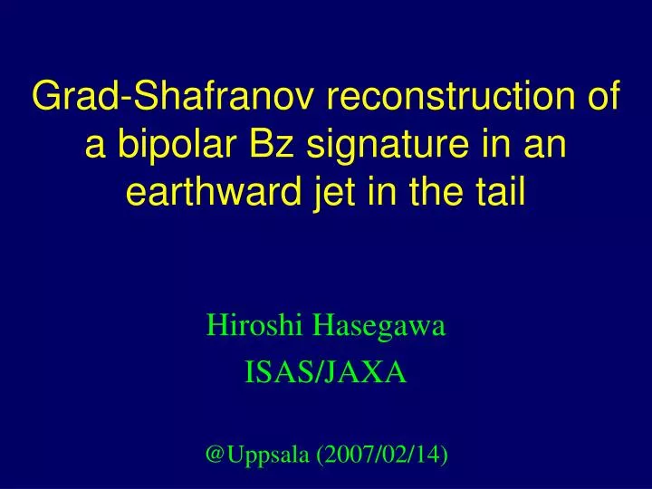
Grad-Shafranov reconstruction of a bipolar Bz signature in an earthward jet in the tail Hiroshi Hasegawa ISAS/JAXA @Uppsala (2007/02/14)
Observation of bipolar Bz + to - Bz (GSM): •in the mid- to distant-tail •along with tailward flows •studied in association with substorms (Ieda et al., 1998, etc.)
Earthward moving flux rope? • - to + Bz •often seen in the near-tail (from Geotail and Cluster observations). Slavin et al. (2003)
Superposed epoch analysis •Core By field •Observed along with earthward flows (BBFs) Slavin et al. (2003)
Models for bipolar Bz in earthward flows Vz •Multiple X-line reconnection(forming magnetic flux ropes) (e.g., Slavin et al., 2003) •Transient reconnection (e.g., Sergeev et al., 1992) •Localized reconnection under guide-field By (Shirataka et al., 2006)
2002-08-13 Cluster event (2200-2400 UT) •Studied by Amm et al. (2006) •associated with a substorm(onset at ~22:50 UT)
2002-08-13 Cluster event (2312-2318 UT) • -/+ Bz embedded in an earthward flow •C3 exactly at the center of the current sheet •C1, 2, 4 on the northern side •Separation ~ 4000 km Bx Bz Vx
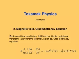
× × Grad-Shafranov reconstruction technique (Hau & Sonnerup, 1999) (A spatial initial value problem) Assumptions Plasma structures are: •in magnetohydrostatic equilibria (time-independent). Magnetic field tension balances with force from the gradient of total (magnetic + plasma) pressure. •2-D (no spatial gradient in the z direction) Grad-Shafranov (GS) equation(e.g., Sturrock, 1994) Pt, p, andBzare functions ofAalone (constant on same field lines).
Reconstruction procedure A 2D structure Reconstruction plane Y Spatial integration Y VST_X X X VST(VHT) (in the x-z plane) Lx = VST_X* T (analyzed interval) X axis: SC trajectory in the x-y plane Z (invariant axis)
Spatial initial value problem (Sonnerup & Guo, 1996) Grad-Shafranov equation spatial integration in -/+y direction (2nd order Taylor exp.) (1st order Taylor exp.) GS eq.
z x cc = 0.961 •Roughly circular flux rope •Flux rope with half width of ~1 Re •Strong core field (mostly By) VHT = (237, 27, 23) km/s in GSM i = (-0.999, 0.042, 0.005) j = (-0.022, -0.621, 0.784) k = (0.036, 0.783, 0.621) Consistent with multiple X-line models?
Z N Y W N X E S S 3D-MHD simulation of localized reconnection with guide-field (Shirataka et al., 2006) guide-field:By0 The Northern hemisphere 2Ry The plane of the equator 2Ry = 3 Re The Southern hemisphere [Slavin et al. 2003]
N W E S Results Reproducing the southward magnetic field Shirataka et al. (2006)
y 11.25Re x 37.5Re -11.25Re Results Virtual S/C obs. in the MHD run Bz[z=0] 11.25Re By0=4nT, 2Ry=3.0Re t=135s
Virtual observation vs real data What will be reconstructed, when applied to the simulation data in which no flux rope is created?
Virtual spacecraft observations @ (x,y,z) = (11.25, 0, 0), (11.25, 0, 1), (11.25, 1, 0), (11.25, 2, 0) Re Applied to the interval T = 105 – 195 s (A suitable model may be determined if the separation is ~2Re. )
GS map recovered from virtual observation Map recovered from data sampled at (x,y,z) = (11.25, 0, 0) Re A flux rope, which does not really exist in the simulation, is reconstructed erroneously. Z(GS) = (0.000, 0.996, 0.087)
Map recovered from data sampled at (x,y,z) = (11.25, 1, 0) Re • The presence of a flux rope-like structure in GS maps does not necessarily mean that it exists in reality. But, are GS results totally meaningless?
Map recovered from data sampled at (x,y,z) = (11.25, 0, 0) Re Simulation result at the time when Bz reversal is at x=11.25 Re (in the same plane)
Map recovered from data sampled at (x,y,z) = (11.25, 1, 0) Re Simulation result at the time when Bz reversal is at x=11.25 Re (in the same plane)
Which model is more reasonable (for the Cluster event)? CL event: •Roughly circular •Pressure minimum at the core Simulation result: • Elongated in the x direction • Enhanced P at the front
Summary •The GS method cannot accurately recover the magnetic topology. One must be cautious about interpretation of model-based (force-free, or GS model) results. •It seems possible to get some information on the basic structure (shape, pressure distribution, etc.) in the reconstruction plane. •The Cluster bipolar Bz event on 2001-08-13 is most likely explained by a flux rope (multiple X-line reconnection). •A suitable separation distance for discriminating models is a few Re (comparable to the jet width).