Download
1 / 21
210 likes | 343 Views
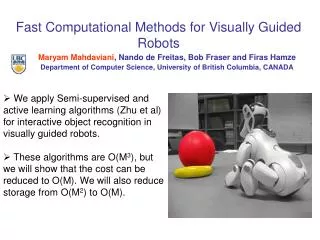
This research presents advancements in semi-supervised and active learning algorithms for interactive object recognition in visually guided robots, reducing computational costs from O(M³) to O(M) and storage from O(M²) to O(M). Leveraging iterative methods like Krylov and the Fast Gauss Transform, we enable real-time pixel labeling and efficient data management. The findings demonstrate Aibo’s ability to recognize multiple objects and prompt user labeling to enhance performance. These methodologies can extend to various applications such as SLAM, segmentation, and ranking.

E N D
Fast Computational Methods for Visually Guided Robots Maryam Mahdaviani, Nando de Freitas, Bob Fraser and Firas Hamze Department of Computer Science, University of British Columbia, CANADA • We apply Semi-supervised and active learning algorithms (Zhu et al) for interactive object recognition in visually guided robots. • These algorithms are O(M3), but we will show that the cost can be reduced to O(M). We will also reduce storage from O(M2) to O(M).
Object recognition with semi-supervised data and simple color features
Aibo is able to identify objects in different settings. Aibo can learn and classify several objects at the same time.
Semi-supervised Learning We want: A full labeling of the data We have: Input data x, two labels yl xi wij xj
Semi-supervised Learning Leads to a Linear System of Equations Differentiating the Error function and equating it to zero, gives the solution in terms of a linear system of equations (Zhu et al, 2003): Where W is the adjacency matrix. 0 0
The big computational bottleneck is M3 Solving the linear system of equations costs O(M3) , where M is a large number of unlabeled features. What is large M?? 1955: M=20 1965: M=200 1980: M=2000 1995: M=20000 2005: M=200000 So over the course of 50 years M has increased by a factor of 104. However, the speed of computers has increased by a factor of 1012. From this, the problematic O(M3) bottleneck is evident.
From O(M3) to O(M2):Krylov Iterative Methods (MINRES) • Using iterative methods (of which Krylov are well known to work best), the cost can be reduced to O(M2) times the number of iterations. The expensive step in each iteration is the following matrix-vector multiplication: • This matrix vector multiplication can be written as two O(M2) Gaussian kernel estimates: • These kernel estimates can be solved in O(M) operations using the Fast Gauss Transform.
Intuition: *L Greengard and V Rokhlin,1987 From O(M2) to O(M):The Fast Gauss Transform Storage requirement is also reduced fromO(M2)toO(M)!!
Predicting Pixel Labels • Once we have labels for M points in our training data, we use a classical kernel discriminant for N test pixels • The cost is O(NM)! • By applying the Fast Gauss Transform the cost can be reduced to O(N+M).
Active Learning • Labeling data is an expensive process. We use active learning to choose what pixels should be labeled automatically. • Active learning calls the semi-supervised learning subroutine at each iteration.
Active learning: asking the right questions • We want the robot to ask the right questions. The robot prompts the user for the labels that will improve its performance the most. Aibo recognizes the ball without a problem. Since the orange ring is close to the ball in colour space, Aibo gets confused and decides to prompt the user for labels.
We managed to reduce computational cost from O(M3) to O(M) and storage requirement from O(M2) to O(M). • Currently we are using more sophisticated features (SIFT) and dual KD-tree recursions methods to deal with high dimensions. • These methods can be applied to other problems such as SLAM, segmentation, ranking and Gaussian Processes. Thank You! Questions?
One solution: Power Method • O(N2) per iteration • But it might take TOO MANY iterations to converge
The Fast Gauss Transform- Reduction of Complexity Straightforward (nested loop)
Krylov Subspace Methods: MINRES Algorithm The cost can be reduced to O(M2) times number of iterations.