Download
1 / 40
420 likes | 646 Views
ANALYSIS OF HEALTHCARE METRICS. By Jesse Whiddon. © 2009 – Jesse Whiddon – All rights reserved. Was There Improvement?. Hospital Data Average LOS (days) % Complications

E N D
ANALYSIS OF HEALTHCARE METRICS By Jesse Whiddon ©2009 – Jesse Whiddon – All rights reserved
Was There Improvement? Hospital Data Average LOS (days) % Complications 2007 (last half) 4.98 4.67% 2008 (first half) 4.59 2.61% Difference 0.39 2.06%
About Metrics • “Metric” is derived from the word “measure”. • Whatever metric you decide to use will depend on the process and whether data can be obtained at steps within that process • Metric should be meaningful and representative enough to judge work, effort, quality, timeliness, and satisfaction.
Metrics • Healthcare metrics are usually in the form of time, count, proportion, costs and evaluation. • Although metrics are made for a number of reasons including control, improvement and compliance, we will focus on improvement.
Example Metrics • Time • Length of stay – days • Time in waiting rooms – hours • Time to process a claim • Time spent assembling patients charts
Example Metrics • Count (Total or Average) • Number of readmits • Number left without being seen • Number of patients with incomplete lab slips • Number of patients contacted • Number of errors occurring in a procedure • Comparative count data
Example Metrics • Proportion • % Complications • % Readmits • % Understaffed • Costs • Cost per case or patient • Total costs of procedures • Total cost of salaries • Savings per case
Example Metrics • Evaluation • Customer surveys • Customer complaints
Metrics – Measuring Improvement • Improvement, as measured with data, is based on comparing for differences in the averages of populations or differences from some standard or target. • And on comparing for statistical differences in variation dispersion (distribution) about means.
Metrics – Parametric vs Nonparametric Analysis • Tests for differences in averages are either parametric or nonparametric. • Parametric tests are considered more powerful in measuring differences in means and can be used to measure differences in the amount of dispersion. • Nonparametric tests can be used to compare non-normal distributions.
Metrics – About Parametric Tests • Parametric tests are based on measurements that have population distributions that are approximately “normal” (bell shaped). • Large samples averages of data from non-normal distributions are normally distributed and are therefore acceptable for parametric testing (central limit theorem) • Small sample averages from non-normal distributions tend to keep approaching normality as the sample size increases.
Metrics – Parametric Restrictions for Differences in Means • The data must be approximately normally distributed. • The variances (measures of normal variation) must be equivalent, at least to an acceptable degree. Note: Parametric testing is more restrictive than the non-normal counterpart.
Transforming Non-normal Data for Parametric Analysis • Data from non-normal distributions can be normalized by transformation. • The most common is logarithmic transformation. • For proportions, the arcsine transformation might be necessary.
Metrics – About Nonparametric Tests • Nonparametric tests are suitable for comparing data from non-normal distributions. • Nonparametric tests rank the data by order of magnitude and compare the medians rather than the means. • Small samples from suspected non-normal population distributions can be compared by nonparametric testing.
Metrics – Nonparametric Tests • Since nonparametric testing is “distribution free”, it is suitable for data that are commonly collected in healthcare that are not normally distributed, such as small sample counts of things, proportions and some measurements. Note: Statistical testing for differences in averages needs to be done, only when distributions overlap and it is not clear if there is truly a difference in the averages.
Guidelines for Choosing Parametric or Nonparametric < 30 > 30 Sample Size? Badly Skewed? Y N Normal? Y N Y Y Increase to 50? Transform? N N T-test (Parametric) N Y Z-Test (Parametric) Transform Data? Mann-Whitney.. (Nonparametric)
Metrics – Parametric Application • Parametric tests • z test for comparing the averages of two large samples (n>30) • t test for comparing the averages of two small samples. • t test for matched pairs. • Minimum requirements for these tests are the average, standard deviation and sample size. Individual tests are preferred in order to confirm normality and some statistical software packages require the individual data for input.
About P Values P-Value is the risk in concluding that a difference exists when in fact it does not. Also known as Type I error or alpha risk. P-Value Risk % Confidence % 0.10 10 90 0.05 5 95 0.01 1 99
Comparing Differences in Means for Large Samples - Minitab Stat>Basic Statistics>2 Sample t Test>Summarized Data Hospital Data – 6 Month LOS 4.98 4.59 Dif 0.39 Sample N Mean StDev SE Mean 1 450 4.98 3.00 0.14 2 465 4.59 3.00 0.14 Difference = mu (1) - mu (2) Estimate for difference: 0.390000 95% CI for difference: (0.000665, 0.779335) T-Test of difference = 0 (vs not =): T-Value = 1.97 P-Value = 0.050 DF = 912
Comparing Differences in Proportions for Large Samples - Minitab Stat>Basis Statistics>2 Proportions>Summarized Data Represents a binomial experiment (independent!) Hospital Data – 6 Month % Complications 4.67 2.61 Dif 2.06 Sample X N Sample p 1 21 450 0.046667 2 12 460 0.026087 Difference = p (1) - p (2) Estimate for difference: 0.0205797 95% CI for difference: (-0.00375035, 0.0449098) Test for difference = 0 (vs not = 0): Z = 1.66 P-Value = 0.097 Note: Events were only 21 and 12 in such a large sample
Metrics – Nonparametric Application • Nonparametric tests commonly used: • Man-Whitney U-test for two unmatched samples. • Kruskal-Wallis for more than two unmatched samples. • Wilcoxon test for matched pairs. • Minimum requirements for these tests are the individual tests (for ranking). • Restrictions - The probability distributions do not have to be normal but must be similar.
Mann-Whitney Application Patients with arthritis have been treated with two different drugs at a clinic based on the preference of physicians. A healthcare worker wants to know if one drug is more effective than the other for pain and chooses patients at random to complete a survey consisting of 10 questions. Each has a scale from 0 to 10, with “0” being “without any pain” and “10” being “extreme pain” (i.e. low score has less overall pain). Scores are as follows: Drug A Drug B 12 34 31 20 20 47 19 31 27 18 10 39 33 25 15 37 23
Mann-Whitney Application Results - Minitab Stat>Nonparametrics>Mann-Whitney Mann-Whitney Test and CI: Drug A, Drug B N Median Drug A 9 20.00 Drug B 8 32.50 Point estimate for ETA1-ETA2 is -10.00 95.1 Percent CI for ETA1-ETA2 is (-20.00,0.00) W = 60.0 Test of ETA1 = ETA2 vs ETA1 not = ETA2 is significant at 0.0485 The test is significant at 0.0483 (adjusted for ties)
Kruskal-Wallis Application A healthcare worker collects the waiting times of five different patients chosen at random from out-patient clinics A, B, C, and D to determine if there are differences between the clinics. A B C D 15 19 23 71 28 47 4 45 17 50 1 56 9 31 9 82 8 12 14 40
Kruskal-Wallis Results - Minitab Stat>Nonparametrics>Kruskal-Wallis Kruskal-Wallis Test on Time Clinics N Median Ave Rank Z A 5 15.000 7.3 -1.40 B 5 31.000 12.4 0.83 C 5 9.000 5.1 -2.36 D 5 56.000 17.2 2.92 Overall 20 10.5 H = 12.56 DF = 3 P = 0.006 H = 12.57 DF = 3 P = 0.006 (adjusted for ties)
Wilcoxon Test for Matched Pairs Application A trial was conducted to evaluate the effects of alcohol on reaction time. Twelve students were chosen at random to consume the same amount of a certain alcoholic beverage. Reaction times (minutes) to complete a complex task was measured before and after the beverage consumption. Results were as follows: A 19.7 19.2 G 15.0 18.2 B 17.4 17.3 H 20.0 18.9 C 16.9 16.6 I 23.0 27.4 D 15.6 21.6 J 20.9 23.2 E 17.4 19.6 K 14.7 22.2 F 17.0 18.2 L 14.8 17.5 Did the alcohol affect the performance?
Wilcoxon Matched Pairs Results - Minitab Calc>Calculator (C1-C2) Stat>Nonparametrics>1 Sample Wilcoxon (Test Median) Wilcoxon Signed Rank Test: C3 Test of median = 0.000000 versus median not = 0.000000 N for Wilcoxon Estimated N Test Statistic P Median C3 11 11 10.0 0.025 -2.175 Note: For Mann-Whitney P = 0.0688
Metrics – Frequencies • Chi-square tests for analyzing frequencies are very useful for things that are counted and classified on nominal scales (categories) such as sex, age-group, blood group type, ethnic origin and so on. Tests commonly used are: • Test for Homogeneity • Goodness of fit • Test of association – Contingency tables
Chi-square Tests • The Test for Homogeneity determines if various counts are consistent with random variation. • Goodness of fit is same as homogeneity test except it compares frequencies against some expected frequency of each according to some rule, theory, etc. • Contingency tables are used with two or more rows of observations to test for association between variables.
Chi-square Homogeneity Test Application There are four standard surgical techniques A, B, C and D being used in a particular type surgery. In order to find out if any one is preferred, 160 randomly selected surgeons were asked which technique he or she preferred. Results were as follows: A B C D • 51 37 33 Is there sufficient evidence to conclude that there is a difference in preferences for the four techniques?
Chi-square Homogeneity Test - Minitab SET C1 39 51 37 33 (Observed values) END SET C2 40 40 40 40 (Expected values) END LET K1=SUM((C1-C2)**2/C2) PRINT K1 CDF K1 K2; CHISQUARE 1. LET K3=1-K2 PRINT K3 Data Display K1 4.50000 (Chi-square statistic) Data Display K3 0.0338949 (P-value) Edit>Command Line Editor
Chi-square Goodness of Fit Test Application Suppose in the previous example of the test for homogeneity, a study had been conducted in the past that concluded that there was a preference among doctors for technique B according to the following percentages: A B C D 20% 40% 20% 20% Does this latest sample of 160 surgeons indicate a change from these percentages?
Chi-square Goodness of Fit - Minitab SET C1 39 51 37 33 (Observed values) END SET C2 32 64 32 32 (Expected values calculated from expected percentages) END LET K1=SUM((C1-C2)**2/C2) PRINT K1 CDF K1 K2; CHISQUARE 3. LET K3=1-K2 PRINT K3 Data Display K1 4.98438 (Chi-square statistic) Data Display K3 0.172945 (P-value) Edit>Command Line Editor
Contingency Table Application In a study of the implications of smoking habits to certain regions, a survey of 252 men from these regions showed the following: Region 1 Region 2 Region 3 Total Non-smokers 55 57 66 178 Smokers 34 24 16 74 Total 89 81 82 Is there an association between smoking and regions?
Contingence Table Results - Minitab Stat>Tables>Chi-Square (Table in Worksheet) Expected counts are printed below observed counts Chi-Square contributions are printed below expected counts C10 C11 C12 Total 1 55 57 66 178 62.87 57.21 57.92 0.984 0.001 1.127 2 34 24 16 74 26.13 23.79 24.08 2.367 0.002 2.711 Total 89 81 82 252 Chi-Sq = 7.192, DF = 2, P-Value = 0.027 (Non-sm) (Observed) (Expected) (Cell Chi-sq) (Smokers) (same) Note: Yates Correction not needed. Total of all cells
Metrics – Sample Size • The larger the sample size, the smaller the differences in averages that can be detected. • Often, the amount of difference in averages that is desired to be detected is balanced against the size of the sample required for this detection and the amount of error that can be tolerated for this detection.
Metrics – Sample Size • However, very small differences in averages can result in large savings in costs, thus making large samples necessary. • On the other hand, there are diminishing returns as the sample size becomes larger and larger.
Subjects Not Covered • Sample size for detecting differences • Sampling methods • All restrictions • Precision • Correlation • Regression • Analysis of variance