Download
1 / 23
230 likes | 535 Views
Part IIA, Paper 1 Consumer and Producer Theory. Lecture 5 Compensating and Equivalent Variation Flavio Toxvaerd. Today’s Outline. Welfare Consumer surplus Equivalent variation Compensating variation Slutsky vs Hicksian substitution. Consumer Surplus and Welfare.

E N D
Part IIA, Paper 1Consumer and Producer Theory Lecture 5 Compensating and Equivalent Variation Flavio Toxvaerd
Today’s Outline • Welfare • Consumer surplus • Equivalent variation • Compensating variation • Slutsky vs Hicksian substitution
Consumer Surplus and Welfare Following a price change,
Consumer Surplus and Welfare p1 a b Marshallian Demand x1
Evaluating Welfare Changes • Consider the situation where the price of good 1 takes one of two values, p1= p01 or p1= p11, while the price of good 2 remains unchanged. • When p1= p01 a consumer with income m will maximise utility subject to her budget constraint, and achieve a level of utility u0= v(p01, p2 , m) (the indirect utility function)
Evaluating Welfare Changes • From duality, and the expenditure function, we also know that e(p01, p2 , u0) = m • Similarly, when p1= p11 we can write u1= v(p11,p2 ,m) and e(p11,p2 ,u1) = m • Now consider e(p01, p2 , u1); this gives the expenditure required to achieve the new level of utility, u1 , at the original set of prices, p01.
This gives the equivalent change in income that would have altered the utility of the consumer by the same amount as the price movement Equivalent Variation EV = e(p01, p2 , u1) - m x2 Evaluated at original prices u1 EV u0 b a x1 m/p11 m/p01
Example 1 • Energy assistance for the elderly: • The Government is concerned about high energy prices facing the elderly over the winter months • Two forms of assistance are proposed: • A subsidy of s percent of the price of energy • A lump sum ‘energy rebate’ paid to all pensioners Which policy should the government adopt?
Example 1 The price subsidy will reduce the effective price of electricity, and so increase demand for electricity from x1(p1,p2,m) to x1(p1(1-s),p2,m). x2 u1 The overall cost of the subsidy will be S=(sp1) x1(p1(1-s),p2,m). EV u0 EV gives the size of a lump sum ‘rebate’ required to make the pensioner indifferent between the rebate and the subsidy x1 m/p1 x1(p1) x1(p1(1-s)) m/p1(1-s)
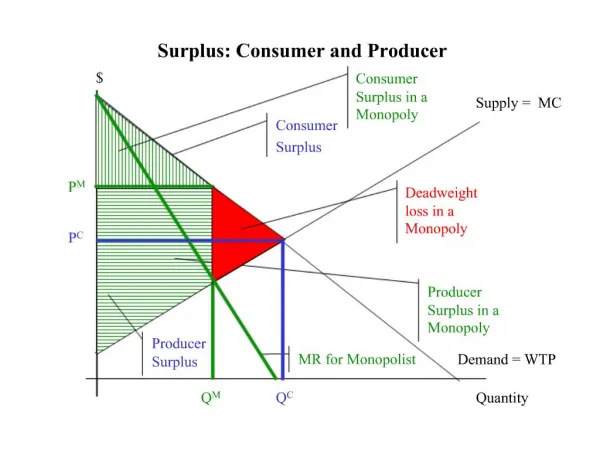
Example 1 So we need to compare the relative magnitudes of S and EV EV is area under Hicksian demand curve at u1
Example 1 p EV = CS if income effect equals zero. EV > CS for price fall of normal good. Hicksian demand p1 Marshallian demand p1(1-s) Recall Slutsky Eqn: x1
Example 1: Subsidy A lump sum rebate is more cost effective than a price subsidy
Example 1: Subsidy p Hicksian demand p1 sp1 subsidy Marshallian demand p1(1-s) x1 x1(p1(1-s),p2,m)
Example 1: Warning! • There are many other important aspects of the problem not addressed in this analysis • This is a ‘partial equilibrium’ analysis. We have not considered: • impact of increased electricity demand on the market price of electricity • impact of any substitution away from alternative heating source • whether or not the government wants to encourage electricity usage by the elderly, and so reduce winter medical care • We have assumed that all consumers are identical - so no consideration of distribution aspects given
Compensating Variation x2 Evaluated at new prices Consider the amount of income a consumer would willingly forsake in exchange for a change in prices. u1 u0 CV CV < 0, positive compensation required CV measures the income effect of a price change x1 m/p10 m/p11
Example 2 • Fixed meal charges • A Cambridge College is considering abandoning the ‘fixed meal charge’ imposed on students, in favour of charging higher food prices ‘in hall’ Should the student union support this proposal?
Example 2 The proposal will increase food prices from p10 to p11. Without any change in student income this will lead to a consumption point, x(p11,p2,m) and utility level u1. x2 The level of income required to compensate the consumer for this price rise will be determined by u0 CV u1 a The student union should support the change if and only if the fixed meal charge is greater than the compensating variation. b x1 m/p11 x11 m/p10 x10
Evaluation • The practical difficulty with this analysis is the measurement of e(p11,p2,u0) • the amount a consumer needs to spend to achieve the original level of utility at the new vector of prices
Passive Expenditure Indirect Effect Actual Expenditure
SlutskyvsHicksian Substitution Hicksian substitutionkeeps utility constant. x2 Slutsky substitutionkeeps ‘real’ income constant, that is - keeps original consumption bundle affordable. u0 u1 Difference is the ‘indirect effect’ x1 x11 m/p10 x10 H.S. S.S.
Example 2, continued The student union can use the present levels of consumption to estimate the compensating variation: Thus, the student union should support the proposal if
Example 2 h(p1,p2,u0) p CV = area under Hicksian demand curve at u0 h(p1,p2,u1) p1 Marshallian demand p1(1-s) x1
Readings • Varian, Intermediate Microeconomics, chapter 14 • Varian, Microeconomic Analysis, chapter 10