Routing
Routing. Routing: Foundations. Task To define the route of packets through the network From the source To the destination system Routing algorithm Defines on which outgoing line an incoming packet will be transmitted Route determination Datagram

Routing
E N D
Presentation Transcript
Routing 1
Routing: Foundations • Task • To define the route of packets through the network • From the source • To the destination system • Routing algorithm • Defines on which outgoing line an incoming packet will be transmitted • Route determination • Datagram • Routing algorithm makes individual decision for each packet • Virtual circuit • Routing algorithm runs only during connect (session routing)
desti- nation link A 0 B 3 C 1 D 4 Data packets Incoming lines Outgoing lines Routing: Routing and Forwarding • Distinction can be made • Routing: makes decision which route to use • Forwarding: what happens when a packet arrives Topology, link utilization, etc. information Router Routing Process Routing table Fills & Updates Uses & Looks up Forwarding Process
Good Properties for Routing Algorithms • Correctness • Simplicity • Minimize load of routers • Robustness • Compensation for IS and link failures • Handling of topology and traffic changes • Stability • Consistent results • No volatile adaptations to new conditions • Fairness • Among different sources compared to each other • Optimality
Routing Algorithms: Conflicting Properties • Often conflicting: fairness and optimization • Some different optimization criteria • Average packet delay • Total throughput • Individual delay • Conflict • Example: • Communication among A A’, B B’, C C’ uses full capacity of horizontal line • Optimized throughput, but • No fairness for X and X’ • Tradeoff between fairness and optimization • Therefore often • Hop minimization per packet • It tends to reduce delays and decreases required bandwidth • Also tends to increase throughput
Classes of Routing Algorithms • Class Non-adaptive Algorithms • Current network state not taken into consideration • Assume average values • All routes are defined off-line before the network is put into operation • No change during operation (static routing) • With knowledge of the overall topology • Spanning tree • Flow-based routing • Without knowledge of the overall topology • Flooding • Class Adaptive Algorithms • Decisions are based on current network state • Measurements / estimates of the topology and the traffic volume • Further sub-classification into • Centralized algorithms • Isolated algorithms • Distributed algorithms
r1 r1 I J K r2’ Optimality Principle and Sink Tree • General statement about optimal routes • If router J is on optimal path from router I to router K • Then the optimal path from router J to router K uses the same route • Example: • r1: route from I to J • r2: route from J to K • If better route r2’ from J to Kwould exist • Then • Concatenation of r1 and r2’ would improve route from I to K • Set of optimal routes • From all sources • To a given destination form a tree rooted at the destination: Sink Tree
B C A D E G J F I N H K L O M Sink Tree Sink Tree for Destination B Subnet • Comments • Tree: no loops • Each optimal route is finite with bounded number of hops • Not necessarily unique • Other trees with same path lengths may exist • Goal of all routing algorithms • Discover and use the sink trees for all routers • Not realistic to use Sink Trees as real-life routing algorithm • Need complete information about topology • Sink Tree is only a benchmark for routing algorithms
Methodology & Metrics • Networks represented as graphs: • Node represents a router • Edge represents a communication line (link) • Compute the shortest path between a given pair of routers • Different metrics for path lengths can be used • Can lead to different results • Sometime even combined (but this leads to computational problems) • Metrics for the "ideal" route, e.g., a "short" route • Number of hops • Geographical distance • Bandwidth • Average data volume • Cost of communication • Delay in queues • ...
Non-Adaptive Routing Shortest Path Routing 10
Non-Adaptive Shortest Path Routing • Static Procedure • Network operator generates tables • Tables • Are loaded when IS operation is initiated and • Will not be changed any more • Characteristics • Simple • Good results with relatively consistent topology and traffic • But • Poor performance if traffic volume or topologies change over time
B C 7 2 3 E 2 3 A D 2 F 1 2 6 2 4 G H Non-Adaptive Shortest Path Routing • Spanning Tree and Optimized Route • Information about the entire network has to be available • i. e. application actually as a benchmark comparison • Example • Link is labeled with distance / weight • Node is labeled with distance from source node along best known path (in parentheses) • Find the shortest path from A to D B (●,-) C (●,-) E (●,-) A D (●,-) F (●,-) G (●,-) H (●,-) 2
Non-Adaptive Shortest Path Routing • Procedure: e. g. according to Dijkstra • Find the shortest path from A to D • Labels may be permanent or tentative • Initially, no paths are known • All nodes are labeled with infinity (tentative) • Discover the labels that represent shortest possible path from source to any node • Make those labels permanent 1. Node A labeled as permanent (filled-in circle) 2. Relabel all directly adjacent nodes with the distance to A(path length, nodes adjacent to source) 3. Examine all tentatively labeled nodes, make the node with the smallest label permanent 4. This node will be the new working node for the iterative procedure(i.e., continue with step 2.)
7 2 3 2 3 2 1 2 6 2 4 Non-Adaptive Shortest Path Routing B (●,-) B (2,A) C (●,-) E (●,-) A D (●,-) F (●,-) G (●,-) G (6,A) H (●,-) • Procedure: e. g. according to Dijkstra • Find the shortest path from A to D: • A flagged as permanent (filled-in circle) • Relabel all directly adjacent nodes with the distance to A • (path length, IS adjacent to the source):
7 2 3 2 3 2 1 2 6 2 4 Non-Adaptive Shortest Path Routing B (2,A) C (●,-) E (●,-) A D (●,-) F (●,-) G (6,A) H (●,-) • Procedure: e. g. according Dijkstra • Find the shortest path from A to D: • ... • Compare all recent, not firmly flagged IS; • flag the one with the lowest number as fixed • This IS is the origin of the iterative procedure • (i. e. continue with item 2.)
7 2 3 2 3 2 1 2 6 2 4 Non-Adaptive Shortest Path Routing C (9,B) B (2,A) C (●,-) E (4,B) E (●,-) A D (●,-) F (●,-) G (6,A) H (●,-) • Procedure: e.g., according to Dijkstra • Find the shortest path from A to D: • Node B has been labeled as permanent (filled-in circle) • relabel all directly adjacent nodes with the distance to B(path length, nodes adjacent to source): • A (does not apply, because it is the origin),
7 2 3 2 3 2 1 2 6 2 4 Non-Adaptive Shortest Path Routing C (9,B) B (2,A) E (4,B) A D (10,H) D (●,-) F (●,-) F (6,E) G (5,E) G (6,A) H (●,-) H (9,G) H (8,F) • Procedure: e.g., according to Dijkstra • find the shortest path from A to D: • … • … • examine all tentatively labeled nodes; • make the node with the smallest label permanent • this node will be the new working node for the iterative procedure ...
Non-Adaptive Routing Flooding 18
Flooding • Principle • IS transmits the received packet to all adjacent IS • But generates "an infinite amount" of packets • Flood limitations • Hop counter in the packet header • Initialize to destination’s distance, or subnet diameter is unknown • Decrement per hop, discard packet at 0 • Keeping history of transferred packets in ISs, delete copies • Source router inserts sequence number into each packet • ISs keeps per-router history of sequence numbers • Old packets are dropped
Selective Flooding • Approach • Do not send out on every line • IS transmits received packet to adjacent stations,located in the Direction of the Destination • With ’regular’ topologies this makes sense and is an optimization • But some topologies do not fit well to this approach • Comment • Geographically-oriented routing got recent interest for mobile scenarios
Flooding • Evaluation and use • In most scenarios impractical because of overhead • Extremely robust • Reaches all ISs • Does not need topology information, no bootstrap • Always finds the shortest path
Adaptive Routing • Class Adaptive Algorithms • Decisions are based on current network state • Measurements / estimates of the topology and the traffic volume • Further sub-classification into • Centralized algorithms • Isolated algorithms • Distributed algorithms
Adaptive Routing Centralized Routing 24
Adaptive Centralized Routing • Principle • One routing control center (RCC) exists in the network • Each IS sends periodically status updates to the RCC • Available neighbors • Current queue length • Line utilization • … • RCC • Collects information • Computes the optimal path each IS pair • Forms routing tables • Distributes tables to ISs
RCC Adaptive Centralized Routing • Characteristics • RCC has complete information • IS is free of routing calculations • But • Re-calculations quite often necessary (approx. once/min or more often) • Low robustness • No correct decisions if network is partitioned • ISs receive tables at different times • Traffic concentration in RCC proximity
Adaptive Routing Isolated Routing 27
Adaptive Isolated Routingthrough Backward Learning • Isolated routing • Every IS makes decision based on locally gathered information only • No exchange of routing information among nodes • Only limited adaptation possibility to changed traffic or topology • IS ‘learns’ from received packets • Source IS • Distance estimate by hop count
Adaptive Isolated Routingthrough Backward Learning • Packet • From source S • received on line L • after C hops S is reachable on L within C hops • Routing table in IS • L - table (destination - IS, outgoing line, Cmin) • Update of the routing table • IS receives packet ( ..., S, C, ... ) on L if not (S in L-Table) then Add(S,L,C) else if C < Cmin then Update(S,L,C)
? ? ? ? Adaptive Isolated Routingthrough Backward Learning • Example: D learns about A • packet ( ..., source - IS, section counter, ...) • P1 ( ..., A, 4, ... ) Add ( A, l1, 4 ) • P2 ( ..., A, 3, ... ) Update ( A, l2, 3 ) I1 A D I2
Adaptive Isolated Routingthrough Backward Learning • Problem • Packets use a different route, e. g. because of failures, high load • Algorithm retains only the old value (because it was "better"), • i. e. algorithm does not react to deteriorations • Solution • Periodic deletion of routing tables(new learning period) • Table deletion • Too often: mainly during the learning phase • Not often enough: reaction to deteriorations too slow
Adaptive Routing Distributed Routing Distance Vector 32
Distance Vector Routing • Distance-Vector Routing • Group of Distance Vector Routing Algorithms • Also known as • Distributed Bellman-Ford algorithm, Ford-Fulkerson algorithm • Use • Was the original ARPANET routing algorithm • Has been used in the Internet as RIP (Routing Information Protocol) • Basic principle • IS maintains table (i.e., vector) stating • Best known distance to destinations • And line to be used • ISs update tables • By exchanging routing information with their neighbors
Distance Vector Routing • Each IS • maintains routing table with one entry per router in the subnet • is assumed to know the ‘distances’ to each neighbor • IS sends list with estimated distances to each destination periodically to its neighbors • X receives list E(Z) from neighbor Y • Distance X to Y: e • Distance Y to Z: E(Z) • Distance X to Z via Y: E(Z)+e • IS computes new routing table from the received listscontaining • Destination IS • Preferred outgoing path • Distance
A I H K A 0 24 20 21 8 A B 12 36 31 28 20 A C 25 18 19 36 D 40 27 8 24 E 14 7 30 22 F 23 20 19 40 G 18 31 6 31 H 17 20 0 19 12 H I 21 0 14 22 10 I J 9 11 7 10 K 24 22 22 0 6 K L 29 33 9 9 Distance Vector Routing line A B C D G 28 I E H F 20 H 17 I 30 I I J K L 18 H 0 - • Previous routing table will not be taken into account • Reaction to deteriorations 15 K JA 8 JI 10 JH 12 JK 6 delay
A B C D E ∞ ∞ ∞ ∞ 1 ∞ ∞ ∞ 1 2 ∞ ∞ 1 2 3 ∞ 1 2 3 4 Distance Vector Routing • Fast route improvement • Fast distribution of information about new short paths (with few hops) • Example • initially A unknown • later: A connected with distance 1 to B, this will be announced • Distribution proportional to topological spread • Synchronous (stepwise) update is a simplification
A B C D E ∞ ∞ ∞ ∞ 3 1 7 3 5 5 7 2 8 2 6 6 4 4 7 5 5 3 3 3 7 6 4 8 6 4 4 6 Distance Vector Routing • Slow distribution of information about new long paths (with many hops) • “Count to Infinity” problem of DVR • Example: deterioration • Here: connection destroyed • A previously known, but now detached • The values are derived from (incorrect) connections of distant IS • Comment • Limit "infinite" to a finite value, depending on the metrics, e.g. • ‘infinite’ = maximum path length+1
A B C D E A ∞ ∞ ∞ ∞ 1 ∞ ∞ ∞ 2 2 ∞ ∞ 3 3 3 ∞ 4 4 4 4 C D B Distance Vector Routing • Variant: ‘Split Horizon Algorithm’ • Objective: improve the "count to infinity" problem • Principle • In general, to publicize the "distance" to each neighbour • If neighbor Y exists on the reported route, X reports the response "false" to Y • distance X (via Y) according to arbitrary i: • Example: deterioration (connection destroyed) • B to C: A = (real),C to B: A = (because A is on path), ... • But: still poor, depending on topology, example • Connection CD is removed • A receives "false information" via B • B receives "false information" via A • Slow distribution (just as before)
Adaptive Routing Distributed Routing Link State Routing 39
Link State Routing • Basic principle • IS measures the "distance" to the directly adjacent IS • Distributes information • Calculates the ideal route • Procedure • Determine the address of adjacent IS • Measure the "distance" (delay, ...) to neighbouring IS • Organize the local link state information in a packet • Distribute the information to all IS • Calculate the route based on the information of all IS • Use • Introduced into the ARPANET in 1979, nowadays most prevalent • IS-IS (Intermediate System-Intermediate System) • developed by DECNET • also used as ISO CLNP in NSFNET • Novell Netware developed its own variation from this (NLSP) • OSPF (Open Shortest Path First) • since 1990 Internet RFC 1247
H H D E D E G G B I B I A C A C F F LAN Link State Routing 1. Phase: gather information about the adjacent intermediate systems
H H D E D E G G B I B I C A A C F F LAN N Link State Routing 1. Phase: gather information about the adjacent intermediate systems Initialization procedure • New IS • Sends a HELLO message over each L2 channel • Adjacent IS • Responds with its own address, unique within the network
Topology, link utilization, etc. information desti- nation link Routing Process A 0 B 3 Routing table Fills & Updates C 1 D 4 ECHO HELLO Link State Routing 2. Phase: measure the "distance" • Definition of distance needed • Usually delay • Where to measure? Router When to start timer? Uses & Looks up Data packets Queues Forwarding Process Incoming lines Outgoing lines
Link State Routing 2. Phase: measure the "distance“ • Queuing delay • Measuring without does not take load into account • Measuring with does usually better • But • Possibility for oscillations (route flapping) • Once per routing table update
Link State Routing 3. Phase: organizing the information as link state packet • Including own address, sequence number, age, "distance" • Timing problems: validity and time of sending • Periodically • In case of major changes
Link State Routing 4. Distributing the local information to all IS • By applying the flooding procedure (very robust) • Therefore sequence number in packets • Problem: inconsistency • Varying states simultaneously available in the network • Indicate and limit the age of packet,i. e. IS removes packets that are too old 5. Computing new routes • Each IS for itself • Possibly larger amount of data available