Download
1 / 68
680 likes | 688 Views
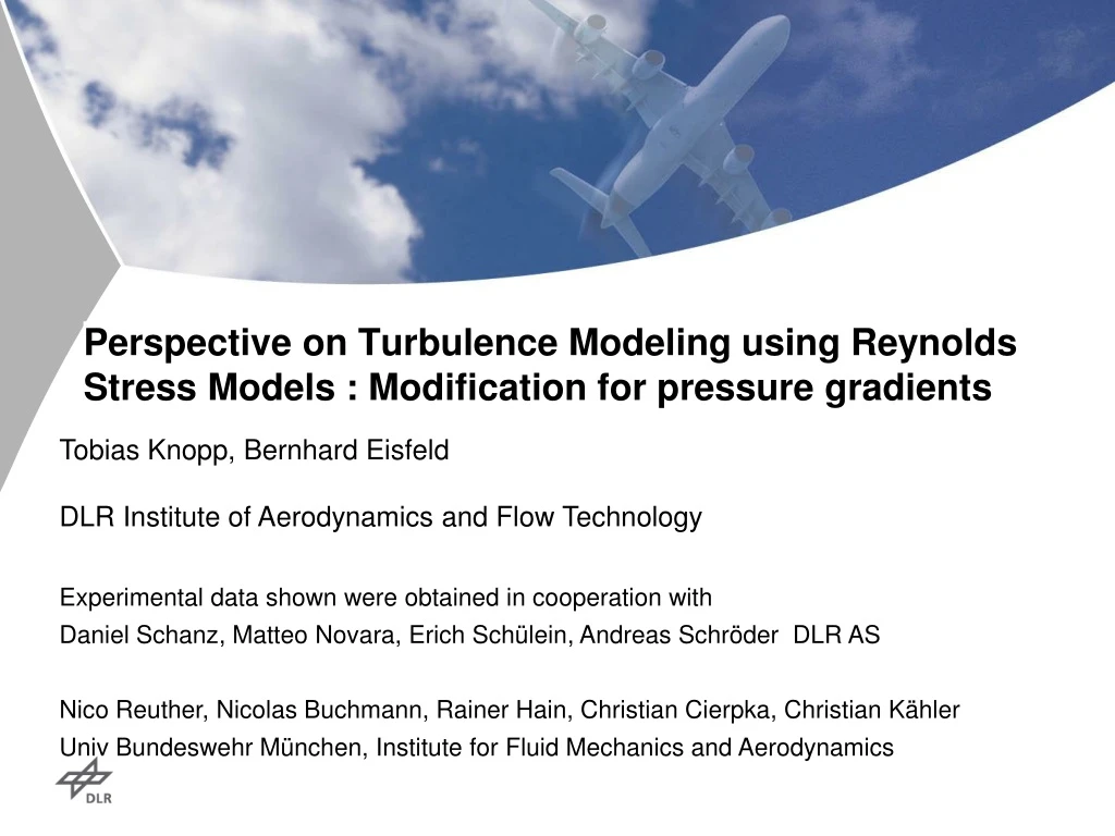
This paper discusses the modification of Reynolds Stress Models for accurate turbulence modeling in the presence of pressure gradients. Experimental data is used to improve the RANS models.

E N D
Perspective on Turbulence Modeling using Reynolds Stress Models : Modification for pressure gradients Tobias Knopp, Bernhard Eisfeld DLR Institute of Aerodynamics and Flow Technology Experimental data shown were obtained in cooperation with Daniel Schanz, Matteo Novara, Erich Schülein, Andreas Schröder DLR AS Nico Reuther, Nicolas Buchmann, Rainer Hain, Christian Cierpka, Christian Kähler Univ Bundeswehr München, Institute for Fluid Mechanics and Aerodynamics
Motivation: Digital aerospace products Numericalsimulationbasedfutureaircraft design Challenges • A/δ99extremely large: large Re and large A • #simulations large for design andoptimization => RANS, not LES
Optimism to describe “first order” steady state aerodynamic flow phenomena within the RANS concept DLR strategy for RANS model improvement Turbulent boundary layers at APG Separation and reattachment Wake flow at APG Interaction of strake vortex and boundary layer at APG Separation in the wing-body junction at APG Interaction of wake flow and boundary layer at APG
DLR strategy for RANS model improvement High-quality database (exp., DNS/LES)
DLR strategy for RANS model improvement High-quality database (exp., DNS/LES) (Empirical) lawsofturbulence
DLR strategy for RANS model improvement High-quality database (exp., DNS/LES) (Empirical) lawsofturbulence Physics-basedimprovementof RANS
DLR strategy for RANS model improvement Surface roughness High-quality database (exp., DNS/LES) Experiments by Nikuradze (Empirical) lawsofturbulence Physicsbasedimprovementof RANS
DLR strategy for RANS model improvement Surface roughness High-quality database (exp., DNS/LES) (Empirical) lawsofturbulence Figure by Aupoix Δu+=f(kr+) kr+ = kruτ / ν Physics-basedimprovementof RANS
DLR strategy for RANS model improvement Surface roughness High-quality database (exp., DNS/LES) (Empirical) lawsofturbulence Physics-basedimprovementof RANS νt = κuτ (y + 0.03kr)
DLR strategy for RANS model improvement Surface roughness High-quality database (exp., DNS/LES) (Empirical) lawsofturbulence Physics-basedimprovementof RANS
DLR strategy for RANS model improvement Turbulent boundary layer at APG High-quality database (exp., DNS/LES) (Empirical) lawsofturbulence Physics-basedimprovementof RANS
DLR strategy for RANS model improvement Turbulent boundary layer at APG High-quality database (exp., DNS/LES) Relevant parameter space? (Empirical) lawsofturbulence Physics-basedimprovementof RANS
Data base set-up: The parameter space Pressure gradient parameter Reynolds number
Data base set-up: The parameter space Pressure gradient parameter A320 flap Reynolds number
Data base set-up: The parameter space A320 flap A380 flap
Data base set-up: The parameter space A380 flap A350 wing A380 wing
Data base set-up: The parameter space DLR institute AS decision 2009: New data needed! Only experiments can give large Re!
Data base set-up: The parameter space Exp I. Assess PIV at moderate Re
Experiment #1 (2011): RETTINA I exp. (DLR + UniBw Munich) Large scaleoverview 2D2C PIV 2D3C PIV LR μPTV U∞= 6 … 12m/s Reθ up to 10000 and δ99 =0.1m Thick boundary layers enable PIV
Data base set-up: The parameter space Exp I. Assess PIV at moderate Re
Data base set-up: The parameter space Exp II. Higher Re
Experiment #2 (2015): RETTINA II exp. (DLR + UniBw Munich) Funded by DLR institute AS and by DFG Defined inflow condition. Defined outflow condition APG region Flow relaxation ZPG Log-law U∞= 10m/s, 23m/s, 36m/s
Experiment #2 (2015): RETTINA II exp. (DLR + UniBw Munich) APG region ZPG Log-law U∞= 36m/s Reθ=41000
Experiment #2 (2015): RETTINA II exp. (DLR + UniBw Munich) Large-scale 2D2C-PIV 9 cams 2D3C PIV micro 2D2C PTV 3D3C PTV STB (shakethe box)
Experiment #2 (2015): RETTINA II exp. (DLR + UniBw Munich) Challenge: Large rangeofscaleof turbulent boundarylayer Solution approach: Multi-resolution multi-camera PIV U=36m/s Reθ=41000 ν/uτ = 20μm δ99 = 0.2m
Experiment #2 (2015): RETTINA II exp. (DLR + UniBw Munich) Challenge: Large rangeofscaleof turbulent boundarylayer Solution approach: Multi-resolution multi-camera PIV U=36m/s Reθ=41000 ν/uτ = 20μm δ99 = 0.2m
Experiment #2 (2015): RETTINA II exp. (DLR + UniBw Munich) Challenge: Large rangeofscaleof turbulent boundarylayer Solution approach: Multi-resolution multi-camera PIV U=36m/s Reθ=41000 ν/uτ = 20μm δ99 = 0.2m
Experiment #2 (2015): RETTINA II exp. (DLR + UniBw Munich) Challenge: Large rangeofscaleof turbulent boundarylayer Solution approach: Multi-resolution multi-camera PIV U=36m/s Reθ=41000 ν/uτ = 20μm δ99 = 0.2m STB=„shake-the-box“ Particle-tracking-approach Schanz, Schröder, Novara @ DLR-AS
Mild separation and reattachment Experiment #3 (August 2017) within DLR internal project
DLR strategy for RANS model improvement High-quality database (exp., DNS/LES) (Empirical) lawsofturbulence Physics-basedimprovementof RANS
Empirical wall law at APG • Mean velocity profiles • 2D2C Reynolds stresses
Empirical wall law at APG Aim: Empirical wall-law at APG for y<0.1δ99 U=36m/s Δpx+=0.015 y<10%δ99
Empirical wall law at APG Aim: Empirical wall-law at APG for y<0.1δ99 U=36m/s Δpx+=0.015 y<10%δ99
Empirical wall law at APG Hypothesis #1: Resilience of a small log-region U=36m/s Δpx+=0.015 y<0.1δ99
Empirical wall law at APG Hypothesis #1: Resilience of a small log-region U=36m/s Δpx+=0.015 Galbraith et al. (1977), Granville (1985), Bradshaw (1995), Perry & Schofield (1973), Durbin & Belcher (1992) Skare & Krogstad (1994) Spalart & Coleman … y<0.1δ99
Results and analysis y+ Ξ-1 =
Empirical wall law at APG U=36m/s Δpx+=0.015 y<0.1δ99
Empirical wall law at APG Hypothesis #2: square-root (sqrt)-law above the log-region Szablewski (1954), Townsend (1961), McDonald (1969), Brown & Joubert … U=36m/s Δpx+=0.015 y<0.1δ99
Results and analysis Hypothesis #2: square-root (sqrt)-law above the log-region U=36m/s Reθ=41000 Δpx+=0.015 y<0.1δ99
Results and analysis Composite profile Brown & Joubert 1969 y+log,max
Results and analysis Hypothesis #3: transition from log-law to sqrt-law depends on Δpx+ (probably more complex …) Composite profile Brown & Joubert 1969 y+log,max
Results and analysis Hypothesis #3: transition from log-law to sqrt-law depends on Δpx+ (probably more complex …) Composite profile Brown & Joubert 1969 y+log,max
Results and analysis Hypothesis #3: transition from log-law to sqrt-law depends on Δpx+ (probably more complex …) ZPG Δpx+→0 Pure log-law
Results and analysis Hypothesis #3: transition from log-law to sqrt-law depends on Δpx+ (probably more complex …) Separation Δpx+→ ∞ Pure sqrt-law (Stratford)
Empirical wall law at APG Hypothesis #4: decrease of log-law slope parameter Ki at APG • Slope coefficient K „von Karman constant“ κ=0.40+/-0.1 ZPG
Empirical wall law at APG Hypothesis #4: decrease of log-law slope parameter Ki at APG • Slope coefficient K „von Karman constant“ κ=0.40+/-0.1 APG ZPG
Empirical wall law at APG Hypothesis #4: decrease of log-law slope parameter Ki at APG • Slope coefficient K „von Karman constant“ κ=0.40+/-0.1 APG
Empirical wall law at APG Hypothesis #4: decrease of log-law slope parameter Ki at APG • Slope coefficient K „von Karman constant“ κ=0.40+/-0.1 APG
DLR strategy for RANS model improvement High-quality database (exp., DNS/LES) (Empirical) lawsofturbulence Physics-basedimprovementof RANS