Download
1 / 37
370 likes | 670 Views
Assessment of Cost of Service to Agriculture Consumers. New Delhi June 17, 2010. Structure of Presentation. Module 1: Introductory. Module 2: Agricultural background of utilities. Module 3: Important Consideration in assessing agriculture CoS.

E N D
Assessment of Cost of Service to Agriculture Consumers New Delhi June 17, 2010
Structure of Presentation Module 1: Introductory Module 2: Agricultural background of utilities Module 3: Important Consideration in assessing agriculture CoS Module 4: Model for determination of cost of service Module 5: Conclusions
Module 1 Introductory
Key objective of the study To formulate methodology to determine the cost of service for agricultural consumers and examination of issues related to it taking into account quality of supply, including hours of supply, voltage fluctuations, reliability of supply etc.
Selection of utilities Utilities selected have significant agricultural load
Approach to the study Selection of Development Finalization Utilities of Model of Model Gujarat In consultation National & International UGVCL with Literature Review PGVCL Andhra Pradesh Standing Developing an Excel Based Committee Model APCPDCL APNPDCL Respective Identification of Data SERC Karnataka Requirements BESCOM Improvising Model with feedback Haryana from FOIR Standing Committee UHBVN
Module 2 Agricultural background of utilities
100% 1% 3% 16% 28% 80% 52% 51% 11% 60% 35% 27% 1% 40% 10% 29% 5% 47% 20% 1% 36% 29% 18% 0% Andhra Pradesh Karnataka Haryana Gujarat States Canals Tanks Tubewells Other wells Other sources 57% 60% 50% 48% 50% 36% 40% 30% 24% 30% 20% 10% 0% APCPDCL APNPDCL BESCOM UGVCL PGVCL UHBVN Power Consumption in Agriculture sector Sources of irrigation in States Tube wells forms important source of irrigation in all states which consumes substantial quantum of power supply. Share of power consumption in agriculture Agriculture sector forms a substantial part of the total power consumed Data sources of 2007/08
Module 3 Important Consideration in assessing agriculture CoS
Important considerations in assessing Agriculture CoS….i • Agriculture gets supply during odd hours of the day • In most cases agriculture category gets supply during odd hours • Few exceptions are there. E.g. UGVCL- Time schedule for supply to agriculture is announced weekly and is divided into various group which receives 8 hours of power during the day on rotational basis • Administered peak for agriculture • Usually agriculture category does not receive round the clock supply. Supply is regulated and rostered leading to “Administered Peak” • Flexibility in usage hours could further increase class peak and coincident peak
Important considerations in assessing Agriculture CoS….ii • Low growth of agriculture power demand • Growth in agriculture consumption lower than other categories • Higher cost of power purchase due to growth of overall demand need not be allocated to agriculture • Poor quality of power supply to agriculture • Often characterised with poor voltage profile and unreliable supply • Tariff design for agriculture consumers should take this into consideration
Important considerations in assessing Agriculture CoS….iii • Diversity in agriculture power demand over the year • Wide variations in demand across seasons &cropping pattern • Methodology to determine CoS to reflect the seasonality in agriculture demand • Estimation of losses incurred in supplying to agriculture category • Agriculture category has substantial unmetered consumption • Losses are not known appropriately (including the breakup in terms of technical and commercial component) • Proper treatment to losses in methodology for assessing CoS
Module 4 Model for determination of cost of service
Functionalisation of Functionalisation of Classification of Costs Classification of Costs : : Costs: Costs: Sample Feeder Data Sample Feeder Data Demand Demand Power Purchase Power Purchase Derivation of Load Curve Derivation of Load Curve Energy Energy Transmission Transmission Class Load Factor Class Load Factor Customer Customer Distribution Distribution Estimation of Coincident Factor Estimation of Coincident Peak Estimation of Coincident Peak Allocation of Costs to Allocation of Costs to agriculture category agriculture category Block Approach Block Approach for assessing for assessing Estimation of Estimation of energy component of power energy component of power Cross Cross Estimation of cost of supply to Estimation of cost of supply to purchase purchase Subsidies Subsidies agriculture consumer category agriculture consumer category Model for Determination of CoS
Information Requirement Utility system load details Power purchase details (base year and relevant year) Energy details of the utility Profit & loss accounts of the utility Balance sheet and its respective schedules of the utility Revenue details of the utility Detailed composition of all costs incurred by the utility Details of technical and commercial losses in agricultural category Voltage level wise classification of cost Load data of the sample feeders • Sources for Data Collection • Secondary sources such as Tariff orders, Profit & Los Accounts, Trial balance, Balance sheet etc. • Discussions with the concerned utilities and State Electricity Regulatory Commission. • Load studies are based on sample survey in consultation with the concerned utilities.
Step 1 - Functionalisation of costs Process of dividing the total cost of the distribution utilities on basis of the functions performed - power purchase, transmission and distribution • Power Purchase Function • All costs related to purchase of power; inclusive of in-house generation cost, power purchase through long term, short term power purchase contracts, trading and unscheduled interface mechanism. • Transmission Function • All costs associated with the transfer of power from power plant to boundaries of utility; predominantly fixed costs • Distribution Function • All costs associated with the transfer of power from the transmission system through the distribution system to the consumer (end user); inclusive of costs incurred by the utility in activities such as R&M, A&G, and employees related expenses etc.
100% 80% 60% 40% 20% 0% APCPDCL APNPDCL BESCOM UGVCL PGVCL UHBVN Power Purchase Transmission Distribution Costs breakup between different functions • Power Purchase costs forms about 75-85% of the total utility cost • Transmission cost forms about 5-10% of the total utility cost • Distribution cost forms about 10-15% of the total utility cost Source: Annual Report of 2007/08 of respective utilities
Step 2 - Classification of costs Explained in next few slides for one utility- UGVCL
Classification of Power Purchase & TransmissionIllustrative example- UGVCL- 2007/08 • Power Purchase cost is classified into fixed and variable costs in the ratio as stated in the tariff order • Transmission cost being fixed in nature is classified as demand cost
Classification of distribution costsIllustrative example- UGVCL Costs related to Distribution function are first classified voltage wise and thereafter based on the nature of costs based on the discussion with the officials of the utility
Classification of distribution costs (in Rs Cr)Illustrative example- UGVCL
Step 3- Sample Feeder Analysis • Identification of sample feeders • Predominantly agriculture load (80%) • Representative of the different circle to capture the geographical spread • Identification of sample days for data collection • 18 days uniformly spread across the entire year to capture the seasonality in agricultural demand of the utility. • 1 day of utility peak day • Derivation of load curve from the above data • Estimation of Class Load Factor • Average Demand/ Peak demand • Estimation of load loss factor • Empirical formula by EPRI to estimate energy losses • (0.3 *Load Factor +0.7 (Load Factor)^2
Step 4 - Estimation of Coincident Factor Coincident factor is the ratio of agricultural demand at the time of the system peak to the agricultural peak demand
Estimation of CF using average peak • Agriculture category faces administered peak with lack of voluntary consumption, thus usage of single peak gives biased results • States witness large variation in monthly peak, thus usage of average peak will capture the overall seasonality during the year. • Steps in Calculating Coincident Factor • Ascertain the time and magnitude of system peak for each of the 12 months separately • Establish the corresponding load from the sample feeder data (average if there are more than two readings for the month) • From the above, take a simple average of above 12 monthly readings. • This average divided by the feeder sample peak gives the CF
Illustration- UGVCL Estimation of CF Selected Days for sample collection Sample Feeder Data for 24 Hours of a day Max feeder load = 9.25 MW CF= Agri demand during system peak/ Max peak = 3.51/9.25 = 37.97%
Step 5 - Estimation of Coincident Peak Estimating Non Coincident Peak When segregated technical and commercial losses available NCP = (Consumption and commercial losses in MU)/(LF*8.76) +(Technical Loss in MU)/(LLF*8.76) When losses could not be segregated into technical and commercial losses NCP = (consumption + total loss)/ (LF*8.76) Coincident peak is the contribution of the agricultural demand to the system peak demand Coincident Peak = Non Coincident peak * Coincident Factor)
Step 6 - Block approach to asses energy component of power purchase cost Different consumer categories pose different weights on the incremental power purchase over the years. Each category should be charged in accordance with their respective share of the incremental power purchase Merit Order Stack for 2007/08 D Growth Block Power purchase over and above the base block Estimate the per unit variable cost for growth block (X2) Variable cost for agri: Incremental Input to agri * X2 C Variable cost of power purchase attributable to agriculture category B Base Block Power Purchase for 2005/06 Estimate the per unit variable cost for base block (X1) Variable cost for agri: Base year Input to agri * X1 A
“Growth Block” “Base Block” Y million kWh X million kWh Illustrative example Cost of PP for Agriculture = Variable cost of base block * X MU + Variable cost of growth block * Y MU (incremental increase in agri sales)
Step 7 - Allocation of classified costs • Allocation of Demand Costs • For all functions demand cost is allocated on basis of coincident peak demand • Allocation of Energy Costs: • For power purchase energy cost component is allocated on the basis of block approach (previous slide) • For transmission & distribution function, energy cost component is allocated on the basis of ratio of agricultural consumption to the total consumption of the utility • Allocation of Customer Costs: • For three functions, customer related cost is allocated on the basis of the ratio of number of agricultural consumers to the total consumers of the utility. Sum total of the different cost (demand, energy and customer related cost) allocated to the agri consumers gives the total cost of supplying power to agricultural consumers as incurred by the particular utility.
Illustration- UGVCL- Allocation of cost In ratio of energy sent to Agricultural consumers to total power purchase On basis of Coincident peak Block approach In ratio of Agricultural consumer to total
Step 7 - Estimation of Cross Subsidies Cross Subsidy to agricultural consumers = Total Cost of supplying power to agri consumers – revenue from sale of power to agri – Subsidy provided by the government Illustrative Example- UGVCL
Module 5 Conclusions
Conclusions……i • Move towards the actual cost to serve pricing principle • It would introduce transparency in rate designing and hence in subsidy/ cross subsidy assessment • Special attention to be taken in allocating power purchase costs • Power purchase costs form significant share (75-80%) in overall costs (fixed and variable) • Further, fixed costs ranges between 20% to 50% of the total PP cost (depending on vintage/type/technology of plant) • Agriculture CoS to also reflect quality and reliability of supply • Reliabity of supply -Agriculture consumers mostly get restricted supply • When consumers pre informed: No discount on cost of supply • When consumers not pre informed: Discount on cost of supply
Conclusions……ii • Quality of supply – Often characterised by poor voltage profile • Modify the total cost of power purchase on account of agriculture consumers considering the average voltage deviations beyond permissible limit • Aggregating the penalty levied on licensees due to poor quality supply and, thereby, moderating the power purchase cost • Use of appropriate load curves • Need of load research study for assessment of power demand of consumer class • Sample feeders selected to have predominant load of agricultural consumers • Need to capture seasonal diversity in estimation of CF • Agriculture demand varies across year due to different seasons, cropping pattern and rainfall
Conclusions……iii • Capture the diversity in agriculture demand by taking into account sample load data spread across the year • Estimation of CF to be based on average monthly peak • Agriculture faces administered peak • Consumption curve for agriculture would be different had they been provided 24hrs access to power • Use of single “peak” for estimating CoS imposes higher burden on this category and does not take into account the effect of seasonality • Need to change the assets/expenditure accounting practices • Utilities should maintain the voltage wise inventory of assets