55:148 Digital Image Processing Chapter 11 3D Vision, Geometry Topics:
420 likes | 596 Views
55:148 Digital Image Processing Chapter 11 3D Vision, Geometry Topics: Basics of projective geometry Points and hyperplanes in projective space Homography Estimating homography from point correspondence The single perspective camera An overview of single camera calibration

55:148 Digital Image Processing Chapter 11 3D Vision, Geometry Topics:
E N D
Presentation Transcript
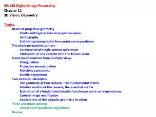
55:148 Digital Image Processing • Chapter 11 3D Vision, Geometry • Topics: • Basics of projective geometry • Points and hyperplanes in projective space • Homography • Estimating homography from point correspondence • The single perspective camera • An overview of single camera calibration • Calibration of one camera from the known scene • Scene reconstruction from multiple views • Triangulation • Projective reconstruction • Matching constraints • Bundle adjustment • Two cameras, stereopsis • The geometry of two cameras. The fundamental matrix • Relative motion of the camera; the essential matrix • Estimation of a fundamental matrix from image point correspondences • Camera Image rectification • Applications of the epipolar geometry in vision • Three and more cameras • Stereo correspondence algorithms • Review
Three cameras and trifocal tensor Three camera matrices: : projection of the optical center on respective camera
Three cameras and trifocal tensor Three camera matrices: : projection of the optical center on respective camera Scene planes derived by three matching projection lines
Three cameras and trifocal tensor Three camera matrices: : projection of the optical center on respective camera Scene planes derived by three matching projection lines Following that the three planes intersect on a common line
Three cameras and trifocal tensorContinued….. Using and We get
Three cameras and trifocal tensorContinued….. Using and We get
Three cameras and trifocal tensorContinued….. Using and We get Leads to Where, for ;
Three cameras and trifocal tensorContinued….. Using and We get Leads to Where, for ; Putting it into
Three cameras and trifocal tensorContinued….. Using and We get Leads to Where, for ; Putting it into Trifocal constraint:
Stereo correspondence algorithms We know how to determine 3D depth using point correspondence after image rectification
Stereo correspondence algorithms We know how to determine 3D depth using point correspondence after image rectification
Stereo correspondence algorithms We know how to determine 3D depth using point correspondence after image rectification So, the problem boils down to solving point correspondence among multiple stereo camera images
Approach Reduce possible candidate pairs of corresponding points using various geometric and photometric constraints
Approach Reduce possible candidate pairs of corresponding points using various geometric and photometric constraints Built point correspondence using “correspondence scoring” and optimization techniques
Approach Reduce possible candidate pairs of corresponding points using various geometric and photometric constraints Built point correspondence using “correspondence scoring” and optimization techniques Different constraints:
Approach Reduce possible candidate pairs of corresponding points using various geometric and photometric constraints Built point correspondence using “correspondence scoring” and optimization techniques Different constraints: Epipolar constraint Uniqueness constraint Symmetry constraint Photometric compatibility constraint Geometry similarity constraint Disparity smoothness constraint Disparity search range Disparity gradient limit Ordering Limit
Feature based stereo correspondence Objective: determine the disparity gradient of a pair of matches and use that to score “goodness” of a matching pair
Feature based stereo correspondence Objective: determine the disparity gradient of a pair of matches and use that to score “goodness” of a matching pair Compute average coordinates as the coordinates of and in the Cyclopean image Determine the cyclopean difference
Feature based stereo correspondence Objective: determine the disparity gradient of a pair of matches and use that to score “goodness” of a matching pair Compute average coordinates as the coordinates of and in the Cyclopean image Determine the cyclopean difference Compute the difference in disparity between the matches of and
Disparity gradient constraint Disparity gradient:
Disparity gradient constraint Disparity gradient: Disparity constraint: Impose a constraint on the disparity gradient measure that should not exceed a preset threshold (say, ‘1’)
Algorithm Extract feature-based points in the left and right images to build the correspondence
Algorithm Extract feature-based points in the left and right images to build the correspondence For each point in the left image, build initial list of correspondence points in the right image
Algorithm Extract feature-based points in the left and right images to build the correspondence For each point in the left image, build initial list of correspondence points in the right image For each possible candidate match, find the number of other possible matches
Algorithm Extract feature-based points in the left and right images to build the correspondence For each point in the left image, build initial list of correspondence points in the right image For each possible candidate match, find the number of other possible matches fulfilling the disparity gradient constraint and use the number as the “likelihood” measure for the candidate match Find the highest scoring match; remove all matches involving any of the two points impose uniqueness constraint
Algorithm Extract feature-based points in the left and right images to build the correspondence For each point in the left image, build initial list of correspondence points in the right image For each possible candidate match, find the number of other possible matches fulfilling the disparity gradient constraint and use the number as the “likelihood” measure for the candidate match Find the highest scoring match; remove all matches involving any of the two points impose uniqueness constraint Repeat Step 2 until all possible matches are established
Review • Basics of projective geometry • Points and hyperplanes in projective space • Perspective projection of parallel lines Properties of projection
Review • Basics of projective geometry • Points and hyperplanes in projective space • Homography • Estimating homography from point correspondence • Homography ≈ Collineation ≈ Projective transformation • is a mapping from one projection plane to another projection plane for the same -dimensional scene and the common origin • Also, expressed as • Property: • Any three collinear points in remain collinear in • Prove! • Method: • Minimize algebraic distance errors (a canonical soln.) • Apply ML estimation
Review • The single perspective camera • An overview of single camera calibration • Calibration of one camera from the known scene • Camera Model • Different coordinate systems • Different transformation matrices • Single camera calibration using • known 3D scene points • Given: a set of image-scene • point correspondences • Output: the projection matrix • Step 1 Initialization using • linear estimation • Step 2 Optimization using • maximum likelihood estimation
Review • Scene reconstruction from multiple views • Triangulation • Projective reconstruction • Matching constraints • Bundle adjustment • Scene reconstruction from multiple views • Task: Given matching points in images. Determine the 3D scene point. • Basic Principle: Back-trace the ray in 3D scene for each image. The scene point is the common intersection of all rays. • Information needed: To back-trace a ray in the scene space, we need to know the corresponding camera matrix .
Review • Two cameras, stereopsis • The geometry of two cameras. • The fundamental matrix • Relative motion of the camera; the essential matrix • Estimation of a fundamental matrix • Applications • Epipolar constraint • Fundamental matrix • First camera • Second camera
Review • Two cameras, stereopsis • The geometry of two cameras. • The fundamental matrix • Relative motion of the camera; the essential matrix • Estimation of a fundamental matrix • Applications • Epipolar lines
Review • Two cameras, stereopsis • The geometry of two cameras. • The fundamental matrix • Relative motion of the camera; the essential matrix • Estimation of a fundamental matrix • Applications • Image Rectification
Review • Two cameras, stereopsis • The geometry of two cameras. • The fundamental matrix • Relative motion of the camera; the essential matrix • Estimation of a fundamental matrix • Applications • Panoramic view
Review • Two cameras, stereopsis • The geometry of two cameras. • The fundamental matrix • Relative motion of the camera; the essential matrix • Estimation of a fundamental matrix • Applications • Panoramic view