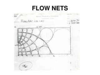
FLOW NETS
FLOW NETS. Techniques for Finding “Solutions” to Groundwater Flow”. Techniques for Finding “Solutions” to Groundwater Flow” Inspection (intuition) Graphical Techniques. Techniques for Finding “Solutions” to Groundwater Flow” Inspection (intuition) Graphical Techniques Analog Models.

FLOW NETS
E N D
Presentation Transcript
Techniques for Finding “Solutions” to Groundwater Flow” • Inspection (intuition) • Graphical Techniques
Techniques for Finding “Solutions” to Groundwater Flow” • Inspection (intuition) • Graphical Techniques • Analog Models
Techniques for Finding “Solutions” to Groundwater Flow” • Inspection (intuition) • Graphical Techniques • Analog Models • Analytical Mathematical Techniques (Calculus)
Techniques for Finding “Solutions” to Groundwater Flow” • Inspection (intuition) • Graphical Techniques • Analog Models • Analytical Mathematical Techniques (Calculus) • Numerical Mathematical Techniques (Computers)
I. Introduction A. Overview
I. Introduction A. Overview • one of the most powerful tools for the analysis of groundwater flow.
I. Introduction A. Overview • one of the most powerful tools for the analysis of groundwater flow. • provides a solution to LaPlaces Equation for 2-D, steady state, boundary value problem.
I. Introduction A. Overview • one of the most powerful tools for the analysis of groundwater flow. • provides a solution to LaPlaces Equation for 2-D, steady state, boundary value problem. • To solve, need to know:
I. Introduction A. Overview • one of the most powerful tools for the analysis of groundwater flow. • provides a solution to LaPlaces Equation for 2-D, steady state, boundary value problem. • To solve, need to know: • have knowledge of the region of flow
I. Introduction A. Overview • one of the most powerful tools for the analysis of groundwater flow. • provides a solution to LaPlaces Equation for 2-D, steady state, boundary value problem. • To solve, need to know: • have knowledge of the region of flow • boundary conditions along the perimeter of the region
To solve, need to know: • have knowledge of the region of flow • boundary conditions along the perimeter of the region • spatial distribution of hydraulic head in region.
Composed of 2 sets of lines • equipotential lines (connect points of equal hydraulic head) • flow lines (pathways of water as it moves through the aquifer.
Composed of 2 sets of lines • equipotential lines (connect points of equal hydraulic head) • flow lines (pathways of water as it moves through the aquifer. d2h + d2h = 0 gives the rate of change of dx2 dy2 h in 2 dimensions
Assumptions Needed For Flow Net Construction • Aquifer is homogeneous, isotropic • Aquifer is saturated
Assumptions Needed For Flow Net Construction • Aquifer is homogeneous, isotropic • Aquifer is saturated • There is no change in head with time
Assumptions Needed For Flow Net Construction • Aquifer is homogeneous, isotropic • Aquifer is saturated • There is no change in head with time • Soil and water are incompressible
Assumptions Needed For Flow Net Construction • Aquifer is homogeneous, isotropic • Aquifer is saturated • there is no change in head with time • soil and water are incompressible • Flow is laminar, and Darcys Law is valid
Assumptions Needed For Flow Net Construction • Aquifer is homogeneous, isotropic • Aquifer is saturated • there is no change in head with time • soil and water are incompressible • flow is laminar, and Darcys Law is valid • All boundary conditions are known.
III. Boundaries A. Types
III. Boundaries • Types 1. Impermeable 2. Constant Head 3. Water Table
III. Boundaries • Types 1. Impermeable 2. Constant Head 3. Water Table
B. Calculating Discharge Using Flow Nets III. Boundaries Q’ = Kph f Where: Q’ = Discharge per unit depth of flow net (L3/t/L) K = Hydraulic Conductivity (L/t) p = number of flow tubes h = head loss (L) f = number of equipotential drops
IV. Refraction of Flow Lines • The derivation • The general relationships • An example problem
IV. Flow Nets: Isotropic, Heterogeneous Types • “Reminder” of the conditions needed to draw a flow net for homogeneous, isotropic conditions • An Example of Iso, Hetero