Download
1 / 20
200 likes | 431 Views
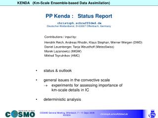
PP Kenda : Status Report christoph.schraff@dwd.de Deutscher Wetterdienst, D-63067 Offenbach, Germany. Contributions / input by: Hendrik Reich, Andreas Rhodin, Klaus Stephan, Werner Wergen (DWD) Daniel Leuenberger, Tanja Weusthoff (MeteoSwiss) Marek Lazanowicz (IMGW)

E N D
PP Kenda : Status Reportchristoph.schraff@dwd.deDeutscher Wetterdienst, D-63067 Offenbach, Germany Contributions / input by: Hendrik Reich, Andreas Rhodin, Klaus Stephan, Werner Wergen (DWD) Daniel Leuenberger, Tanja Weusthoff (MeteoSwiss) Marek Lazanowicz (IMGW) Mikhail Tsyrulnikov (HMC) • status & outlook • general issues in the convective scale experiments for assessing importance of km-scale details in IC • deterministic analysis
Task 1: General issues in the convective scale and evaluation of COSMO-DE-EPS Purpose: Guides decision how resources will be spent on/ split betw. LETKF and SIR (COSMO-NWS and universities); part of the learning process main disadvantage of LETKF: assumes Gaussian error distributions Task 1.1.A: investigate non-Gaussianity by means of O – B statistics (convective / larger scales, different forecast lead times): provides an upper limit estimate of the non-Gaussianity to deal with Task 1.2: investigate non-Gaussianity by examining perturbations of very-short range (2009) forecasts from COSMO-DE-EPS talk by Daniel Leuenberger: Statistical characteristics of high-resolution COSMO Ensemble forecasts in view of Data Assimilation
Task 1.4: M. Tsyrulnikov: Review on Hunt et al. implementation of LETKF difficulty of assimilating non-local satellite data and achieving good resolution in local analysis talk by Breogan Gomez: Single-column experiments on the vertical localisation in the LETKF RWWRP / THORPEX Workshop on 4D-Var and EnKF intercomparison • we should continue with KENDA (LETKF) as planned (4DVAR / EnKF ok for HR DA: everybody pushes the way further on the current road; ensemble size stable (30 – 40); synergistic approaches) • worthwhile to obtain options for EnKF implementations which also make use of 3DVar (by implementing tasks 2.1 , 2.5) • model errors a (the) key issue for advanced DA important for DA to work on model improvement
Task 1.1 D: assess importance of km-scale details versus larger-scale conditions in the IC (do we have to analyse the small scales, or is it sufficient to analyse the large scales, as e.g. incremental 4DVAR (ECMWF) would do ?) Comparison: ‘IEU’: IC from interpolated COSMO-EU analysis of ass. cycle (no LHN) ‘IDE’: IC from COSMO-DE analysis of ass. cycle (no LHN) ‘LHN’: IC from COSMO-DE analysis of ass. cycle (IDE + LHN for use of radar- derived precipitation) Note: – IC from assimilation cycle → late cut-off, very similar set of observations – identical correlation functions (scales) used in nudging for IEU and IDE – identical soil moisture, taken from IEU (with variational soil moisture initialisation) – model version as operational in summer 2009 Period: 31 May – 13 June 2007: air mass convection
31.05. – 13.06.07: air-mass convection 00 UTC runs 06 UTC runs LHN IDE (no-LHN) IEU (coarse IC) LHN IDE (no-LHN) IEU (coarse IC) ETS 0.1 mm FBI # radar ‘obs’ with rain time of day time of day
31.05. – 13.06.07: air-mass convection 00 UTC runs 06 UTC runs LHN IDE (no-LHN) IEU (coarse IC) LHN IDE (no-LHN) IEU (coarse IC) ETS 1 mm FBI # radar ‘obs’ with rain time of day time of day
31.05. – 13.06.07: air-mass convection 12 UTC runs 18 UTC runs 12 18 LHN IDE (no-LHN) IEU (coarse IC) ETS 0.1 mm FBI LHN IDE (no-LHN) IEU (coarse IC) # radar ‘obs’ with rain time of day time of day
31.05. – 13.06.07: air-mass convection 12 UTC runs 18 UTC runs LHN IDE (no-LHN) IEU (coarse IC) LHN IDE (no-LHN) IEU (coarse IC) ETS 1 mm FBI # radar ‘obs’ with rain time of day time of day
Examples radar (12-h sum) IEU (coarse IC) LHN (fine-scale IC) 12-UTC runs, 6 – 18 h fcsts. (nighttime precipitation) 10 June 18 UTC – 11 June 06 UTC 2007 4 June 18 UTC – 5 June 06 UTC 2007
Task 1.1.D: assess importance of km-scale details Results of comparison to coarse-scale ‘IEU’ : • ‘IDE’ better than ‘IEU’ for 12- and 18-UTC runs up to +15h (similar FBI, higher ETS) similar for 0- and 6-UTC runs • improvement by LHN during first 6 hours • ‘LHN’ has better precipitation patterns (6 – 18 h forecast) than ‘IEU’ in some cases Radar With LHN Without LHN (dashed: determininistic) Past experiments (Leuenberger): environment affects impact of fine-scale details in analysis from LHN
Task 2: Technical implementation of an ensemble data assimilation framework / LETKF analysis step (LETKF) outside COSMO code ensemble of independent COSMO runs up to next analysis time separate analysis step code, LETKF included in 3DVAR code of DWD
( - ) + = ( - ) + = ( - ) + = ( - ) + = ( - ) + = → analysis (mean) and analysis error covariance : columns of and in model space : → analysis ensemble member : LOCAL Ensemble Transform Kalman Filter (LETKF)(chart based on a slide of Neil Bowler, UK MetOffice) 0.9 Pert 1 -0.1 Pert 2 -0.1 Pert 3 -0.1 Pert 4 -0.1 Pert 5 (local, inflated) transform matrix Wa perturbed forecasts – ensemble mean forecast analysis mean perturbed analyses = background perturbations Xb → flow-dep. backgr. error covar. analysis error covariance in the (5-dimensional) sub-space S spanned by background perturbations : (linearise obs operator around the mean of ensemble of simulations of an obs) explicit solution for minimisation of cost function (Hunt et al., 2007)
determ. Kalman gain / analysis increments not optimal, if deterministic run (strongly) deviates from analysis mean of ensemble Analysis for a deterministic forecast run : use Kalman Gain K of analysis mean K is already computed in the (L)ETKF ; if the resolution of the deterministic run is higher than of ensemble, the analysis increments have to be interpolated to the fine grid
Task 2.2: almost finished Task 2.4: not yet done read obs (NetCDF) + Grib analysis of ensemble member compute obs–fg (obs. increm.) + QC (contains obs operator) write NetCDF feedback files (obs + obs–fg + QC flags) + Grib files (model) COSMO Task 2.3: finished exp. system read ensemble of NetCDF feedback files + ensemble of COSMO S-R forecast Grib files perform LETKF (based on obs–fg values around each grid pt., calc. transformation matrices and analysis (mean & pert.)) (adapt: C-grid, specific variables (w), efficiency) write ensemble of COSMO S-R analysis Grib files + NetCDF feedback files with additional QC flags ( verif.) LETKF However: scripts written to do a few stand-alone cycles with LETKF → preliminary tests can start soon
NetCDF feedback y, qf, d y qf NetCDF observation write feed- back read obs y qf H(x) read feedback x QC H GRIB H(x) read grib new tool (included in 3DVar code) y: observations x: model state d = y – H(x): innovation H: observation operator qf: quality flag QC: quality control need to include NetCDF observation QC H & in ‘stat’ module common codes in COSMO & ‘stat’ tool Verification / diagnostics: new ‘stat’ tool : compute model (forecast) – obs , as input for verification want have capability of computing distance of model (ensemble member) to observations that have not been used previously in a COSMO run ( SIRF)
Task 2: Technical implementation of an ensemble data assimilation framework / LETKF for verification: ‘stat’-module: compute model (forecast) – obs : adapt verification mode of 3DVar/LETKF package Advantages: – COSMO obs operators available in 3DVAR/LETKF environment 3DVar/ EnKF approaches requiring 3DVar in principle applicable to COSMO LETKF for ICON will require COSMO obs operators in the future – 1 common code for GME/ICON and COSMO to produce input for diagnostics / verif.. Disadvantages: – more complex code for this diagnostic task – possibly additional transformation from COSMO data structure into 3DVAR data structure and vice versa required for new COSMO obs operators. Task 2.1: extract from COSMO: - ‘library 2’ : in progress - ‘library 1’ : finished Task 2.5: - in progress: include above libraries in 3DVar environment, (translate COSMO data structure into 3DVar data structure and vice versa) - not yet started: extend flow control (e.g. reading several Grib files and temporal interpolat.) observation operators H with QC modules for reading obs from NetCDF Task 2.6: Adapt ensemble-related diagnostic tools : not yet started
Task 3: Evaluate and tune LETKF address primary scientific issues related to the LETKF on the convective scale (using only in-situ data at first) • investigate / control noise, adapt in view of non-hydrostatic aspects if mixing of hydrostatically balanced model states (ensemble forecasts) varies with height (vertical localisation), the resulting model analysis will usually not be hydrostatically balanced → get version that can be used to do first tests with radar radial winds • primary scientific issues: – model model (physical) perturbations – multiplicative covariance inflation – localisation (multi-scale DA) – additive covariance inflation with red noise, backscatter, statistical forecast error covariances (‘3DVAR-B’) ‘ – bias removal – noise control (update frequency, digital filter initialisation, lateral boundary cond.) – (convection initiation (warm bubbles, LHN)
Task 4: Inclusion of additional observations Research funded by DWD to develop suitably sophisticated + efficient observation operators for radar data (radial winds + (3-dim.) reflectivity) (Blahak + 2 PhD’s) Task 4.1: Radar radial winds: • implement simple obs operator, then test and tune • particular issues: obs error variances and correlations, superobbing, thinning, localisation Task 4.2: Radar reflectivity (after 2010): Task 4.3: Ground-based GPS slant path delay (after 2010): • particular issue: localisation for non-local obs Task 4.4: Cloud info based on satellite and conventional data (DWD: applied for Eumetsat fellowship, start end of 2010) • derive incomplete cloud analysis, use obs increments of cloud or humidity • use SEVIRI brightness temperature directly in LETKF in cloudy (+ cloud-free) conditions Task 5: Sequential importance resampling (SIR) filter research projects continue within DAQUA (MeteoSwiss investigating on norms)
time SREPS (pred.) SREPS (ass.) … … select best members ( ≤10 ) radar / satellite / in-situ obs. free forecast HRES final weighting after free forecast is computed Weighting + Resampling Guiding steps Weighting + Resampling set up (G-) SIRFtest with COPS period Evaluate classical and spatial (object oriented, fuzzy) metrics for weighting mesoscale (SREPS) and km-scale ensemble members (DLR, MCH) • assess correlation of metrics betw. models of different res. • assess persistence of skill in different metrics Set up standard and G-SIRF with and without standard data assimilation (MIUB, DWD) • assess impact of conventional DA (LHN, PIB) on ensemble development (spread generation, keeping ensemble on track) • implement optimal stepping to a new driving mesoscale ensemble