Download
1 / 20
200 likes | 309 Views
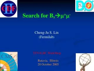
Search for B s m + m - Cheng-Ju S. Lin (Fermilab ) TEV4LHC WorkShop Batavia, Illinois 20 October 2005. Outline. Overall motivations B d,s m + m - Search strategy at CDF and D0 Impact of current results on some SUSY models CDF+D0 projection Some thoughts on LHC. 2.

E N D
Search for Bsm+m- Cheng-Ju S. Lin (Fermilab) TEV4LHC WorkShop Batavia, Illinois 20 October 2005
Outline • Overall motivations • Bd,s m+m- Search strategy at CDF and D0 • Impact of current results on some SUSY models • CDF+D0 projection • Some thoughts on LHC 2
Introduction • In the Standard Model, the FCNC decay of B m+m- is heavily • suppressed SM prediction (Buchalla & Buras, Misiak & Urban) • SM prediction is below the sensitivity of current experiments • (CDF+D0): SM Expect to see 0 events at the Tevatron Any signal would indicate new physics!!
BEYOND STANDARD MODEL m b R-parity violating SUSY ~ n l’i23 l i22 m s • In many SUSY models, the BR could be enhanced by many • orders of magnitude: • For examples: • - MSSM: Br(Bmm) is proportional • to tan6b. BR could be as large as • ~100 times the SM prediction • - Tree level diagram is allowed in • R-parity violating (RPV) SUSY • models. Possible to observe decay • even for low value of tanb. • In context of mSUGRA, Br(Bmm) search complements • direct SUSY searches: (A. Dedes et al, hep-ph/0207026) • Low tan(b) observation of trilepton events • Large tan(b) observation of Br(Bmm)
Data Sample • Both CDF (~360pb-1) and D0 (~300pb-1) use di-muon • trigger sample for the search • Trigger is a vital part of this analysis • Combinatorial background from the raw sample is enormous CDF D0 Search region
Ingredients of the Analysis Overall picture: - Reconstructing di-muon events in the B mass window - Measure the branching ratio or set a limit Normalized to BJ/y K decays Key elements in the analysis: - Construct discriminant to select Bs signal and suppress bkg CDF Likelihood ratio discriminant D0 Cut based analysis - understanding the background - accurately measure the acceptance and efficiency ratios Analysis optimization (figure of merit): CDF expected 90% C.L. upper limit D0 S/(1+sqrt(B))
CDF D0 Central Muon Extension (0.6< |h| < 1.0) Central Muon Chambers (|h| < 0.6) Muon Chambers (|h| < 2.0) GOOD MUON COVERAGE HELPS!!! 7
Reconstruct Normalization Mode (B+J/y K+) CDF D0 central-central muons GOOD MASS RESOLUTION HELPS!!! 8
cut cut B mm Optimization (CDF) • Chosen three primary discriminating variables: • proper decay length (l) • Pointing (Da) |fB – fvtx| • Isolation (Iso) 9
B mm Optimization (D0) signal background • Similar three primary discriminating variables • D0 use 2d lifetime variables instead of 3d • Optimize using MC for signal, data sidebands for background • Random grid search, optimizing for ~ S/(1+sqrt(B)) 10
Likelihood Ratio Discriminant (CDF) • First iteration of analysis used standard cuts optimization • Second iteration uses the more powerful likelihood discriminant • i: index over all discriminating variables • Psig/bkg(xi): probability for event to be signal / background for a given measured xi • Obtain probably density functions of variables using • background: Data sidebands • signal: Pythia Monte Carlo sample 11
Optimization (CDF) Likelihood ratio discriminant: Optimize likelihood and pt(B) for best 90% C.L. limit • Bayesian approach • consider statistical and systematic errors • Assume 1fb-1 integrated luminosity 12
Results CDF D0 • Expected background:4.3 1.2 • Observed: 4 CDF and D0 Combined: • Expected background:1.5 0.2 • Observed: 0 BR(Bsmm) < 1.2×10⁻⁷ @ 90% CL < 1.5×10⁻⁷ @ 95% CL BR(Bdmm) < 3.2×10⁻⁸ @ 90% CL < 4.0×10⁻⁸ @ 95% CL 13
M16=3TeV, mA=700 GeV SO(10) Grand Unification Model R. Dermisek et al., hep-ph/0507233 (2005) R. Dermisek et al., JHEP 0304 (2003) 037 Red regions are excluded by either theory or experiments Green region is the WMAP preferred region Blue dashed line is the Br(Bsmm) contour Light blue region excluded by old Bsmm analysis tan(b)~50 constrained by unification of Yukawa couplings
mSUGRA M0 vs M1/2 Dedes, Dreiner, Nierste, PRL 87(2001) 251804 Excluded • For mh~115GeV implies • 10-8<Br(Bsmm)<3×10⁻⁷ M0 [GeV] Excluded Solid red = excluded by theory or experiment Dashed red line = light Higgs mass (mh) Dashed green line = (dam)susy (in units of 10-10) Black line = Br(Bsmm)
TEVATRON REACH on Bsmm Can push down to Low 10-8 region Still a factor of 10 from SM value
Some Thoughts on LHC • Still a window of opportunity for discovery at the • Tevatron. However, LHC will sweep the measurement. • Maintaining a healthy B physics trigger will be a challenge • at the LHC. It’s all too easy to raise pT threshold and/or • prescale B triggers when trigger rate is high. • Not clear to me how reliable is the background estimate • in various LHC Bsmm projections. Don’t be surprised • if your background turns out to be x10 higher. • Similar search strategy as Tevatron can probably be • adopted at LHC. May require additional discriminating • variables or more sophisticated approach (e.g. NN) • to suppress bkg.
Remaining Thoughts on LHC • Bhh (where h=kaon,pion) will be an issue at LHC. Will • need to have a detailed understanding of muon fake rates. • Some efficiencies may have to be estimated from • Monte Carlo (e.g. isolation cut) need a reliable LHC MC. • Looking forward to the first physics (hopefully surprises) from • the LHC!!
LH CMU-CMU CMU-CMX cut pred obsv pred obsv >0.50 236+/-4 235 172+/-3 168 OS- >0.90 37+/-1 32 33+/-1 36 >0.99 2.8+/-0.2 2 3.6+/-0.2 3 >0.50 2.3+/-0.2 0 2.8+/-0.3 3 SS+ >0.90 0.25+/-0.03 0 0.44+/-0.04 0 >0.99 <0.10 0 <0.10 0 >0.50 2.7+/-0.2 1 3.7+/-0.3 4 SS- >0.90 0.35+/-0.03 0 0.63+/-0.06 0 >0.99 <0.10 0 <0.10 0 >0.50 84+/-2 84 21+/-1 19 FM+ >0.90 14.2+/-0.4 10 3.9+/-0.2 3 >0.99 1.0+/-0.1 2 0.41+/-0.03 0 Background estimate (CDF) 1.) OS- : opposite-charge dimuon, l < 0 2.) SS+ : same-charge dimuon, l > 0 3.) SS- : same-charge dimuon, l < 0 4.) FM : fake muon sample (at least one leg failed muon stub chi2 cut) 20